感知器
问题描述
感知器是二分类的线性分类模型。输入为分类对象的特殊诊断向量,输出为,用于区分分类对象的类型。这有点抽象,所以这里有一个例子。
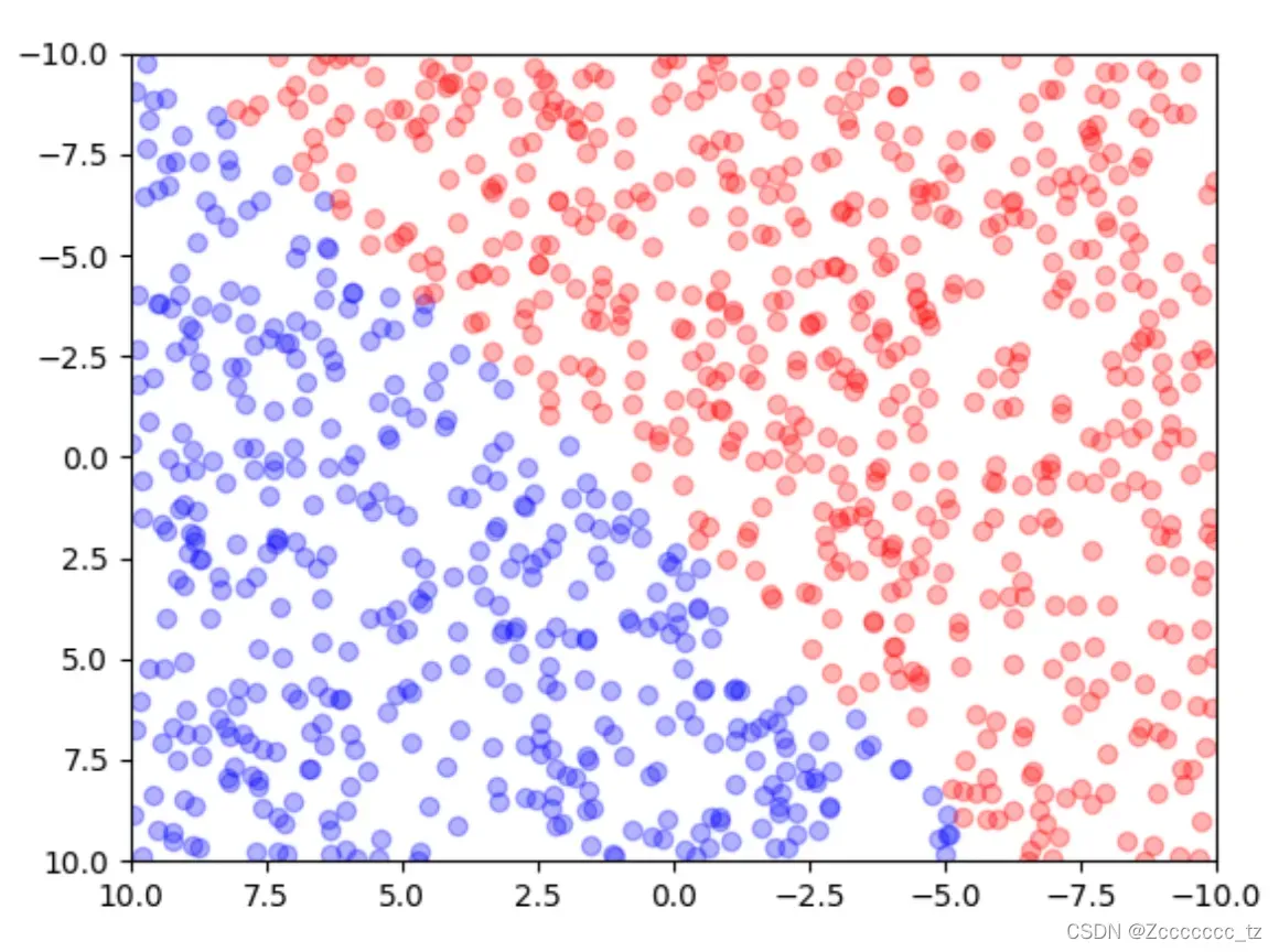
如上图,
- 上图对应的例子就是每个点
- 实例的特征向量指的是这些点的横坐标和纵坐标,我们记为
。
- 我们根据每个点的颜色将点标记为
和
,这就是我们的输出
。
使用这些已知坐标的红蓝点,我们需要训练以下模型,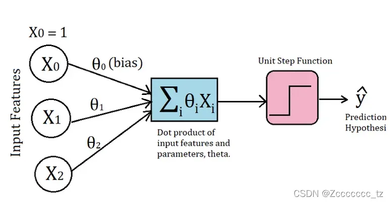
该模型共有参数
,使其能够实现以下功能:
- 当
时,我们知道该点是红色的。
- 当
时,我们知道该点是蓝色的。
在
数据集构建
在开始之前,我们需要自己的整个数据集进行训练。
先导入一些需要的包
import numpy as np
import matplotlib.pyplot as plt
import random
from typing import List, Tuple
然后是时候构建我们的数据集了。
# 随机生成一些点,并根据直线将点划分为2个区域
def sample_point(w: float, b: float, num: int) -> Tuple[List[List[float]], List[float]]:
    x, y = [], []
    for _ in range(num):
        p_x1 = np.random.random_sample(1) * 20 - 10
        p_x2 = np.random.random_sample(1) * 20 - 10
        p_y = 1 if w * p_x1 + b - p_x2 > 0 else -1
        x.append([p_x1, p_x2])
        y.append(p_y)

    return x, y

# 先随机生成一条直线
w_ideal = np.random.random_sample(1) * 10 - 5
b_ideal = np.random.random_sample(1) * 10 - 5

x = np.linspace(-10, 10, 1000)
line_ideal = w_ideal * x + b_ideal
# 搭建数据集
sample_x, sample_y = sample_point(w_ideal, b_ideal, 500)
为了更直观,我们可以用matplotlib可视化这些点
# 可视化
plt.xlim(xmax=-10, xmin=10)
plt.ylim(ymax=-10, ymin=10)
plt.plot(x, line_ideal, 'g', linewidth=10)
for i, p_x in enumerate(sample_x):
    if sample_y[i] == 1:
        plt.scatter(p_x[0], p_x[1], c='r', alpha=0.3)
    else:
        plt.scatter(p_x[0], p_x[1], c='b', alpha=0.3)
plt.show()
我们会得到下面的图片,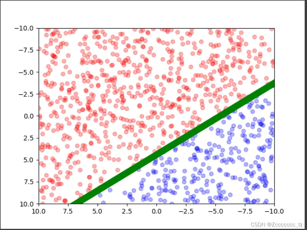
绿线是实际中可以区分红蓝点的直线。
接下来我们要做的就是在代码中假装不知道这一行的参数,即w_ideal和b_ideal,看看能否从数据集中得到我们估计的参数,即w_est和b_ideal。
(可能有人要问了,我们上面不是说三个参数吗?怎么又变成了估计两个参数?别急,后面会介绍)。
模型训练
模型训练的理论支持
回到我们的问题,如何根据点的横纵坐标对点的颜色进行分类?
为了能够实现这个预测功能,我们知道我们需要训练参数
。
假设我们现在有这样一组参数,如何衡量这组参数的好坏?如果这组参数不够好,我们该如何优化这些参数呢?
因此,我们需要定义一个损失函数来衡量这个参数的好坏,并利用损失函数的梯度来最小化损失函数。
损失函数的定义
直观地说,一组好的参数不应该错误分类一个点,因此使用错误分类点的数量作为损失函数是一个合理的想法。那么误分类点有哪些特点呢?
对于第个样本,
- 当样本点为蓝色时,
,被误归为红色,即
。
- 当样本点为红色时,
被误归为蓝色,即
。
总之,我们的损失函数定义为
其中,是误分类点的集合,
。
使用损失函数优化参数
感知器学习算法是错误分类驱动的,特别是使用随机梯度下降。我们首先随机选择一组参数,然后使用梯度下降不断最小化目标函数。
- 这里的最小化过程不是一次将所有错误分类点的梯度下降,而是一次随机选择一个错误分类点,使其梯度下降
- 随机选择一个误分类点,利用该点优化参数
是学习率,取值范围是
Python代码的实现
def perceptron(x, y, lr, t) -> Tuple[np.ndarray, List[int]]:
	"""
	x: 点坐标
	y: 理想输出,+1 或 -1
	lr: learning rate, 学习率
	t: 参数优化次数
	返回:训练完的参数,每次优化前误分类点的个数
	"""
	# 初始化参数
    theta = np.zeros((len(x[0])+1, 1))
    error_list = []  # 误分点列表

    # 开始训练
    for _ in range(t):
        error_count = 0
        error_index = []
        for i, x_i in enumerate(x):
            y_i = theta[0] * x_i[0] + theta[1] * x_i[1] + theta[2]
            # 如果该点被分类错误
            if y_i * y[i] <= 0:
                error_index.append(i)
                error_count += 1
            # print(theta)
        error_list.append(error_count)
        # 随机选取一个误分类点进行参数优化
        if error_count > 0:
            i = random.choice(error_index)
            theta[0] += lr * y[i] * x[i][0]
            theta[1] += lr * y[i] * x[i][1]
            theta[2] += lr * y[i] * 1

    return theta, error_list
调用perceptron函数可以完成我们感知器的训练,得到一组合适的参数,我们可以将其转换成直线参数,转换公式如下:
并与我们的理想线参数进行比较(如果样本点较少,可能与理想线有较大差距。那是因为对于这个样本,区分红蓝点的线不是唯一的)。
然后我们可视化数据,代码如下:
# 根据数据集得到参数
theta, error_list = perceptron(sample_x, sample_y, 0.5, 100)

# 可视化
plt.rcParams['figure.figsize'] = (12.0, 4.0)
plt.subplot(121)
plt.xlim(xmax=-10, xmin=10)
plt.ylim(ymax=-10, ymin=10)
# plt.plot(x, y_ideal)
for i, p_x in enumerate(sample_x):
    if sample_y[i] == 1:
        plt.scatter(p_x[0], p_x[1], c='r', alpha=0.3)
    else:
        plt.scatter(p_x[0], p_x[1], c='b', alpha=0.3)
# 将 theta 转换为直线参数,绘制图像
w_est = - theta[0] / theta[1]
b_est = - theta[2] / theta[1]
print("the estimation of parameter are \n", w_est, "\n", b_est)
y_est = w_est * x + b_est
plt.plot(x, y_est, 'g', linewidth=10)

plt.subplot(122)
plt.plot(np.arange(len(error_list)), error_list, 'g+-')
plt.show()
得到下面的图片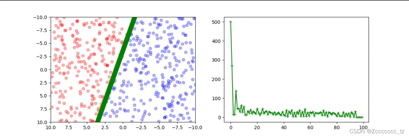
可以看出,绿线很好地将红点和蓝点分开。
如果性能不好(意味着最后仍然有大量点被错误分类),可以通过修改学习率和优化次数得到更准确的模型。
完整的实验代码
import numpy as np
import matplotlib.pyplot as plt
import random
from typing import List, Tuple


def sample_point(w: float, b: float, num: int) -> Tuple[List[List[float]], List[float]]:
    x, y = [], []
    for _ in range(num):
        p_x1 = np.random.random_sample(1) * 20 - 10
        p_x2 = np.random.random_sample(1) * 20 - 10
        p_y = 1 if w * p_x1 + b - p_x2 > 0 else -1
        x.append([p_x1, p_x2])
        y.append(p_y)

    return x, y


def perceptron(x, y, lr, t) -> Tuple[np.ndarray, List[int]]:

    theta = np.zeros((len(x[0])+1, 1))
    error_list = []  # 误分点列表

    # 开始训练
    for _ in range(t):
        error_count = 0
        error_index = []
        for i, x_i in enumerate(x):
            y_i = theta[0] * x_i[0] + theta[1] * x_i[1] + theta[2]
            # 如果该点被分类错误
            if y_i * y[i] <= 0:
                error_index.append(i)
                error_count += 1
            # print(theta)
        error_list.append(error_count)
        if error_count > 0:
            i = random.choice(error_index)
            theta[0] += lr * y[i] * x[i][0]
            theta[1] += lr * y[i] * x[i][1]
            theta[2] += lr * y[i]

    return theta, error_list


def all_code():
    # 生成散点图
    w_ideal = np.random.random_sample(1) * 10 - 5
    b_ideal = np.random.random_sample(1) * 10 - 5
    print("the ideal parameter are \n", w_ideal, "\n", b_ideal)

    x = np.linspace(-10, 10, 1000)
    # line_ideal = w_ideal * x + b_ideal
    # 搭建数据集
    sample_x, sample_y = sample_point(w_ideal, b_ideal, 500)

    # 根据数据集得到参数
    theta, error_list = perceptron(sample_x, sample_y, 0.5, 100)

    # 可视化
    plt.rcParams['figure.figsize'] = (12.0, 4.0)
    plt.subplot(121)
    plt.xlim(xmax=-10, xmin=10)
    plt.ylim(ymax=-10, ymin=10)
    # plt.plot(x, y_ideal)
    for i, p_x in enumerate(sample_x):
        if sample_y[i] == 1:
            plt.scatter(p_x[0], p_x[1], c='r', alpha=0.3)
        else:
            plt.scatter(p_x[0], p_x[1], c='b', alpha=0.3)
    w_est = - theta[0] / theta[1]
    b_est = - theta[2] / theta[1]
    print("the estimation of parameter are \n", w_est, "\n", b_est)
    y_est = w_est * x + b_est
    plt.plot(x, y_est, 'g', linewidth=10)

    plt.subplot(122)
    plt.plot(np.arange(len(error_list)), error_list, 'g+-')
    plt.show()


if __name__ == '__main__':
    all_code()
参考
- “统计学习方法”
- Implementing the Perceptron Algorithm in Python
文章出处登录后可见!