1.从零开始搭建神经网络——不使用框架(纯手撕)
神经网络从0开始
在不使用框架的情况下从头开始实现神经网络,逐步推理应该会加深您对神经网络的理解。
网络结构为三层全连接网络,节点个数依次为784、250、10。对mnist手写数字实现分类。这里minist数据集为csv形式,分训练集和测试集。
1.定义网络结构参数
这里面节点个数比较好理解,重点在于weight_itoh 和weight_htoo 两个矩阵权重。np.random.rand(self.hidden_nodes, self.input_nodes)代表生成self.hidden_nodes行self.input_nodes列的服从0~1的均匀分布的矩阵(左闭右开[0,1))。
class NN:
    def __init__(self, input_nodes, hidden_nodes, output_nodes, lr):
        '''初始化输入节点个数、隐藏层节点个数、输出层节点个数、学习率'''
        self.input_nodes = input_nodes
        self.hidden_nodes = hidden_nodes
        self.output_nodes = output_nodes
        self.lr = lr
        '''初始化权重矩阵,我们有两个矩阵:一个是weight_itoh表示输入层与中间层之间的链路权重形成的矩阵
        一个是weight_htoo表示中间层与输出层之间的链路权重形成的矩阵'''
        self.weight_itoh = np.random.rand(self.hidden_nodes, self.input_nodes)-0.5
        self.weight_htoo = np.random.rand(self.output_nodes, self.hidden_nodes)-0.5
        '''sigmoid激活函数:激活每个节点,得到结果作为信号输入到下一层'''
        self.activation = lambda x: scipy.special.expit(x)
下面主要讲解权重矩阵的参数设置:
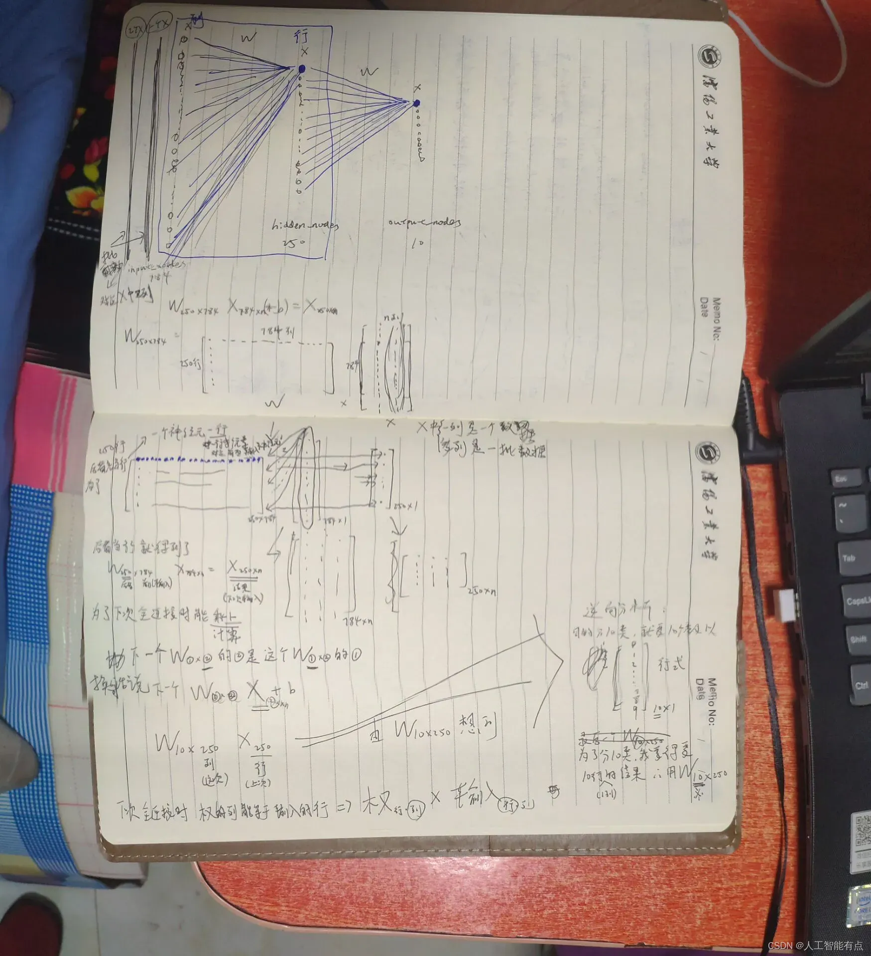
主函数的初始化情况是:第一层网络节点是784个,第二层网络节点是250个,第三层网络节点是10个。那为什么第一个权重矩阵的shape是(250,784)而不是(784,250)呢?这是由全连接运算的规律决定的。
全连接运算公式:Wx + b。在第一次运算(也就是隐藏层接受来自输入层的信号量)中,这个接受的意思可以理解为做了一次全连接即Wx + b,W的shape是(250,784),x的shape是(784,n)。这里n我不太确定暂且先把n理解为批大小。这样一来全连接运算np.dot(self.weight_itoh, x)中的两个矩阵参数的乘法就符合线性代数的规律了,即矩阵A和B相乘要想得到AB的条件是A的列数要等于B的行数,可见self.weight_itoh的列数为784并且x的行数为784,矩阵相乘得到隐藏层的输入hidden_input的shape为(250,n)。然后hidden_input经过隐藏层激活函数得到隐藏层输出hidden_output,激活不改变shape。
隐藏层输出shape为(250,n)。刚刚是输入层->隐藏层,有了隐藏层的输出,现在到了隐藏层->输出层。过程是类似的,隐藏层到输出层的全连接Wx + b,W的shape是(10,250),x是上面的hidden_output它的shape为(250,n),满足矩阵乘法运算。最后输出的是输出层的输入,shape为(10,n)。最后还剩下一个输出层的激活,激活不改变shape。
通过上面的运算过程,可以了解到,输入数据是可以有输出的,不会出现错误。而且最后输出的 shape 为(10,n),满足10分类的结果要求。
上面的分析正确。反之,让我们辩证地瞅瞅,回到最初的疑问:为什么第一个权重矩阵的 shape 是(250,784)而不是(784,250)呢?很简单呀,因为输入x的维度是(784,n),没办法做全连接呢。
总结一个共性,也许你已经发现了。权重矩阵 在全连接网络中,权重矩阵的权重就是同一矩阵中相邻两层节点之间的连接线上的所有数字的组合,总数是个数的乘积前后两层的节点。具体来说,后一层可以理解为一行,前一层可以理解为一列。权重矩阵第一行的系数是连接后一层的第一个节点到第一层的每个节点的线上的系数。同理,权重矩阵第二行的系数就是下一层的第二个节点和第一层的每个节点的连接上的系数……直到权重矩阵的最后一行的系数是最后一个下一层的节点,分别。连接第一层中每个节点的线上的系数。
输入的数据x是很多个列组合在一起的矩阵。x的行是第一层节点的个数,按这个说法来讲,好像也只有第一层节点个数作为权重矩阵的列,全连接才具有可解释性。
一个全连接过程的结果的 shape 是后面一层的节点个数作为行。这个结果经过激活作为下一个全连接的输入时,下一个全连接的W的行(是本个全连接后面一层的节点个数)与列(本个全连接前面一层的个数,也是x的行数)具备和之前的结果相乘的条件。
总之,这件事是正确理解的。画的通俗易懂,文字后面的附图(很潦草……),做动画就好了,但是我不会做动画。 . .
到目前为止,我认为最重要的一点已经结束。
2.神经网络的推理
推理:使用实时数据进行前向传播(不会反向传播)。使用经过训练的神经网络来预测未知数据。
class NN:

    '''
    接着我们先看forward函数的实现,它接收输入数据,通过神经网络的层层计算后,在输出层输出最终结果。
    输入数据要依次经过输入层,中间层,和输出层,并且在每层的节点中还得执行激活函数以便形成对下一层节点的输出信号。
    我们知道可以通过矩阵运算把这一系列复杂的运算流程给统一起来。'''
    def reasoning(self, x):
        # 根据输入数据计算并输出答案
        # 计算中间层从输入层接收到的信号量
        hidden_input = np.dot(self.weight_itoh, x)
        # 计算中间层经过激活函数后形成的输出信号量
        hidden_output = self.activation(hidden_input)  # 激活
        # 计算结束层从中间层接受的信号量
        final_input = np.dot(self.weight_htoo, hidden_output)
        # 计算最外层神经元(结束层)经过激活函数后形成的输出信号量
        finnal_output = self.activation(final_input)
        return finnal_output
np.dot(x,y),当x,y都是二维时是矩阵乘法,代表x*y。
3.训练
这里的权重矩阵更新使用推导公式,暂时没必要理解。理解的关键在于上面的参数设置。以后框架会直接调用优化器自动更新,这里就不用多说了,除非你想清楚。
class NN:

    def train(self, train_data, train_label):
        # forward 正向传播
        hidden_input = np.dot(self.weight_itoh, train_data)
        hidden_output = self.activation(hidden_input)
        finnal_input = np.dot(self.weight_htoo, hidden_output)
        final_output = self.activation(finnal_input)
        # calculate error 计算每层的误差
        output_errors = train_label - final_output
        hidden_errors = np.dot(self.weight_htoo.T, output_errors * final_output * (1 - final_output))
        # backward 反向传播(更新参数中的公式求导可以不用理解)
        self.weight_htoo += self.lr * np.dot((output_errors * final_output * (1 - final_output)), np.transpose(hidden_output))
        self.weight_itoh += self.lr * np.dot((hidden_errors * hidden_output * (1 - hidden_output)), np.transpose(train_data))
        pass
4.主函数
if __name__ == '__main__':

    # 应为输入图片具有 28*28=784 个像素点,所以网络的输入层要具备784个节点
    # 分为10类,所以网络的输出层要具备10个节点
    input_nodes = 784
    hidden_nodes = 250
    output_nodes = 10
    lr = 0.1
    net = NN(input_nodes, hidden_nodes, output_nodes, lr)

    # 读取数据集文件,存入内存,关闭文件
    datafile = open("./dataset/mnist_train.csv")
    data = datafile.readlines()
    datafile.close()

    epochs = 10
    # 10轮训练
    for epoch in range(epochs):
        for record in data:
            # 预处理数据
            # 归一化:/255防止为0链路更新出现问题,+0.01使结果处于 0.01~1 中
            # 转换为numpy支持的二维矩阵
            label_and_input = record.split(',')
            train_data = np.asfarray(label_and_input[1:])/255.0 * 0.99 + 0.01
            train_data = np.array(train_data, ndmin=2).T  # shape(784,1)

            # label 设置图片与数值的对应关系
            train_label = np.zeros(output_nodes)
            train_label[int(label_and_input[0])] = 1
            train_label = np.array(train_label, ndmin=2).T  # shape(10,1)

            net.train(train_data=train_data, train_label=train_label)
            # prediction = net.forward(train_data)
            # train_error = prediction - train_label


    # 测试
    datafile = open("./dataset/mnist_test.csv")
    data = datafile.readlines()
    datafile.close()

    score = []
    for record in data:
        # 预处理数字图片
        all_value = record.split(',')
        input = np.asfarray(all_value[1:])/255*0.99+0.01  # shape(784,)
        input = np.array(input, ndmin=2).T  # shape(784,1)

        correct_number = int(all_value[0])
        print('该图片对应的数字是:', correct_number)
        # 网络推理数字图片 对应的数字
        predict = net.reasoning(input)
        # 找到数值最大的神经元对应的编号
        predict = np.argmax(predict)
        # 这里的argmax返回的是索引,只不过此时索引和图片数字相同,都是0~9,所以输出网络预测可以用预测的索引
        print('网络认为图片的数字是:', predict)
        if predict == correct_number:
            score.append(1)
        else:
            score.append(0)
    print(score)
    print('correct rate:', np.array(score).sum()/len(score))
结果:
该图片对应的数字是: 7
网络认为图片的数字是: 7
该图片对应的数字是: 2
网络认为图片的数字是: 5
该图片对应的数字是: 1
网络认为图片的数字是: 1
该图片对应的数字是: 0
网络认为图片的数字是: 0
该图片对应的数字是: 4
网络认为图片的数字是: 4
该图片对应的数字是: 1
网络认为图片的数字是: 1
该图片对应的数字是: 4
网络认为图片的数字是: 4
该图片对应的数字是: 9
网络认为图片的数字是: 3
该图片对应的数字是: 5
网络认为图片的数字是: 4
该图片对应的数字是: 9
网络认为图片的数字是: 7
[1, 0, 1, 1, 1, 1, 1, 0, 0, 0]
correct rate: 0.6
完整代码如下
链接:下载数据集
提取码:9zxm
import numpy as np
import scipy.special


class NN:
    def __init__(self, input_nodes, hidden_nodes, output_nodes, lr):
        # 输入节点个数 隐藏层节点个数 输出层节点个数 学习率
        self.input_nodes = input_nodes
        self.hidden_nodes = hidden_nodes
        self.output_nodes = output_nodes
        self.lr = lr
        '''初始化权重矩阵,我们有两个矩阵:一个是weight_itoh表示输入层与中间层之间的链路权重形成的矩阵
        一个是weight_htoo表示中间层与输出层之间的链路权重形成的矩阵'''
        self.weight_itoh = np.random.rand(self.hidden_nodes, self.input_nodes)-0.5
        self.weight_htoo = np.random.rand(self.output_nodes, self.hidden_nodes)-0.5
        '''sigmoid激活函数:激活每个节点,得到结果作为信号输入到下一层'''
        self.activation = lambda x: scipy.special.expit(x)

    '''接着我们先看forward函数的实现,它接收输入数据,通过神经网络的层层计算后,在输出层输出最终结果。
    输入数据要依次经过输入层,中间层,和输出层,并且在每层的节点中还得执行激活函数以便形成对下一层节点的输出信号。
    我们知道可以通过矩阵运算把这一系列复杂的运算流程给统一起来。'''
    def reasoning(self, x):
        # 根据输入数据计算并输出答案
        # 计算中间层从输入层接收到的信号量
        hidden_input = np.dot(self.weight_itoh, x)
        # 计算中间层经过激活函数后形成的输出信号量
        hidden_output = self.activation(hidden_input)  # 激活
        # 计算结束层从中间层接受的信号量
        final_input = np.dot(self.weight_htoo, hidden_output)
        # 计算最外层神经元(结束层)经过激活函数后形成的输出信号量
        finnal_output = self.activation(final_input)
        return finnal_output

    def train(self, train_data, train_label):
        # forward 正向传播
        hidden_input = np.dot(self.weight_itoh, train_data)
        hidden_output = self.activation(hidden_input)
        finnal_input = np.dot(self.weight_htoo, hidden_output)
        final_output = self.activation(finnal_input)
        # calculate error 计算每层的误差
        output_errors = train_label - final_output
        hidden_errors = np.dot(self.weight_htoo.T, output_errors * final_output * (1 - final_output))
        # backward 反向传播
        self.weight_htoo += self.lr * np.dot((output_errors * final_output * (1 - final_output)), np.transpose(hidden_output))
        self.weight_itoh += self.lr * np.dot((hidden_errors * hidden_output * (1 - hidden_output)), np.transpose(train_data))
        pass

if __name__ == '__main__':
    # nn = NN(3, 3, 3, .1)
    # nn.forward([1,9,6])
    # train

    input_nodes = 784
    hidden_nodes = 250
    output_nodes = 10
    lr = 0.1

    datafile = open("./dataset/mnist_train.csv")
    data = datafile.readlines()
    datafile.close()
    # print(len(data[0]))
    # count_list = []
    # for i in data:
    #     count_list.append(len(i.split(',')))
    # print(count_list)

    net = NN(input_nodes, hidden_nodes, output_nodes, lr)

    epochs = 10
    for epoch in range(epochs):
        for record in data:
            # 预处理数据
            # 归一化:/255防止为0链路更新出现问题,+0.01使结果处于 0.01~1 中
            # 转换为numpy支持的二维矩阵
            label_and_input = record.split(',')
            train_data = np.asfarray(label_and_input[1:])/255.0 * 0.99 + 0.01
            train_data = np.array(train_data, ndmin=2).T  # shape(784,1)

            # label 设置图片与数值的对应关系
            train_label = np.zeros(output_nodes)
            train_label[int(label_and_input[0])] = 1
            train_label = np.array(train_label, ndmin=2).T  # shape(10,1)

            net.train(train_data=train_data, train_label=train_label)
            # prediction = net.forward(train_data)
            # train_error = prediction - train_label

    # 测试
    datafile = open("./dataset/mnist_test.csv")
    data = datafile.readlines()
    datafile.close()
    score = []
    for record in data:
        # 预处理数字图片
        all_value = record.split(',')
        input = np.asfarray(all_value[1:])/255*0.99+0.01  # shape(784,)
        input = np.array(input, ndmin=2).T  # shape(784,1)

        correct_number = int(all_value[0])
        print('该图片对应的数字是:', correct_number)
        # 网络推理数字图片 对应的数字
        predict = net.reasoning(input)
        # 找到数值最大的神经元对应的编号
        predict = np.argmax(predict)
        # 这里的argmax返回的是索引,只不过此时索引和图片数字相同,都是0~9,所以输出网络预测可以用预测的索引
        print('网络认为图片的数字是:', predict)
        if predict == correct_number:
            score.append(1)
        else:
            score.append(0)
    print(score)
    print('correct rate:', np.array(score).sum()/len(score))
附录
绘图分析-图形分析
附录下的一些小demo都是一些python基础语法,不用看,写了纯粹是因为自己懵懵懂懂,记录一下。精华在上面。
np.random.rand()返回一个一组服从[0,1)均匀分布的随机样本值
weight_htoo = np.random.rand(3, 4)
print(weight_htoo)
print(type(weight_htoo))
[[0.50615296 0.43160166 0.02933226 0.20085878]
 [0.02680242 0.02659778 0.96719308 0.79753404]
 [0.06243989 0.35310816 0.77511554 0.18622354]]
<class 'numpy.ndarray'>
np.zeros()
a = np.zeros(10)
print(a)
print(type(a))
[0. 0. 0. 0. 0. 0. 0. 0. 0. 0.]
<class 'numpy.ndarray'>
train_data = [i for i in range(1, 10)]
print(train_data, type(train_data))
train_data = np.asfarray(train_data)
print(train_data, type(train_data))

train_data2 = np.array(train_data, ndmin=2).T
print(train_data2, type(train_data2), train_data2.shape)
train_data3 = np.array(train_data, ndmin=3).T
print(train_data3, type(train_data3), train_data3.shape)
[1, 2, 3, 4, 5, 6, 7, 8, 9] <class 'list'>
[1. 2. 3. 4. 5. 6. 7. 8. 9.] <class 'numpy.ndarray'>
[[1.]
 [2.]
 [3.]
 [4.]
 [5.]
 [6.]
 [7.]
 [8.]
 [9.]] <class 'numpy.ndarray'> (9, 1)
[[[1.]]

 [[2.]]

 [[3.]]

 [[4.]]

 [[5.]]

 [[6.]]

 [[7.]]

 [[8.]]

 [[9.]]] <class 'numpy.ndarray'> (9, 1, 1)
np.dot(x,y)情况多种。x,y都是二维时,是矩阵乘法,规则同线性代数。
[外链图片转存失败,源站可能有防盗链机制,建议将图片保存下来直接上传(img-1o1zRlfZ-1647842980538)(photo/QQ图片20220319222025.jpg)]
import numpy as np

import matplotlib.pyplot as plt

# 定义数据: 使用numpy生成200个随机点
x_data = np.linspace(-0.5, 0.5, 200)

print(x_data, type(x_data), x_data.shape)

x_data = x_data[:, np.newaxis]

print(x_data, type(x_data), x_data.shape)
结果:
E:\Anaconda3\envs\tf1.14\python.exe D:/CodeField/Python/BaDou/9第八周作业/tests.py
[-0.5        -0.49497487 -0.48994975 -0.48492462 -0.4798995  -0.47487437
 -0.46984925 -0.46482412 -0.45979899 -0.45477387 -0.44974874 -0.44472362
      .            .           .           .           .           .
      .            .           .           .           .           .
      .            .           .           .           .           .
  0.43467337  0.43969849  0.44472362  0.44974874  0.45477387  0.45979899
  0.46482412  0.46984925  0.47487437  0.4798995   0.48492462  0.48994975
  0.49497487  0.5       ] <class 'numpy.ndarray'> (200,)
[[-0.5       ]
 [-0.49497487]
 [-0.48994975]
 [-0.48492462]
      ...
 [ 0.48492462]
 [ 0.48994975]
 [ 0.49497487]
 [ 0.5       ]] <class 'numpy.ndarray'> (200, 1)

Process finished with exit code 0

         .
  0.43467337  0.43969849  0.44472362  0.44974874  0.45477387  0.45979899
  0.46482412  0.46984925  0.47487437  0.4798995   0.48492462  0.48994975
  0.49497487  0.5       ] <class 'numpy.ndarray'> (200,)
[[-0.5       ]
 [-0.49497487]
 [-0.48994975]
 [-0.48492462]
      ...
 [ 0.48492462]
 [ 0.48994975]
 [ 0.49497487]
 [ 0.5       ]] <class 'numpy.ndarray'> (200, 1)

Process finished with exit code 0
文章出处登录后可见!