入门机器学习(西瓜书+南瓜书)神经网络总结(python代码实现)
1. 神经网络
1.1 通俗理解
这一次的内容比较难理解。因此,作者试图明确什么是常用词中的神经网络?他是怎么到这里的?为什么这几年这么火?基于此的深度学习发生了什么?让我们一步一步地揭开神经网络的神秘面纱。
神经网络模型其实起源于众所周知的线性模型,是的,你没听错。很简单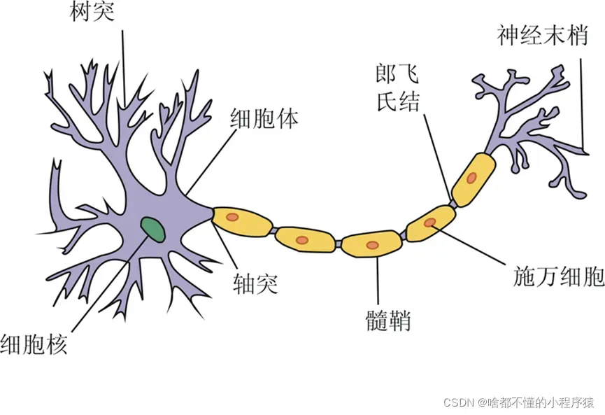
没关系,不擅长生物的同学看不懂上面的说法。科学家们对结构进行了简化,根据神经元的结构构建了下图所示的感知器模型。这也是神经网络的早期原型。公式表达也是线性关系的组合,是最简单的单层神经网络,包括输入、权重和输出。这个神经元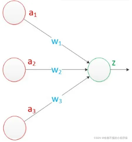
这就是最为原始的神经网络,也就是感知机(perceptron),早在1957年,由罗森布拉特发明,后期的神经网络与支持向量机都是以此为基础进行的,而感知机的基本原理就是逐点修正,首先在平面上随意取一条分类线,统计分类错误的点;然后随机对某个错误点就行修正,即变换直线的位置,使该错误点得以正确分类;接着再随机选择一个错误点进行纠正,分类线不断变化,直到所有的点都完全分类正确了,就得到了最佳的分类线。
但是,到了1969年,马文明斯基提出了针对感知机难以解决的“异或”问题,和感知机数据线性不可分的情形导致感知机进入10年的冷静期。
到了1974年,Werbos首次提出把BP算法应用到神经网络,也就是多层感知机(Multilayer Perception,MLP)也叫做人工神经网络(Artificial Neural Network,ANN)。是一个带有单隐层的神经网络。而随着神经网络的隐藏层出现,以及对激活函数的改进,多层感知机成功的解决了异或问题。
再到后来随着自动链式求导理论的发展,神经网络之父,Hinton成功的把使用BP(Back Propagation)算法来训练神经网络。
为了简化神经网络以减少神经网络中需要确定的大量参数,在1995年,YannLeCun(杨立坤)提出了著名的卷积神经网络(Conventional Neural Network,CNN),神经网络实现了局部连接,权重共享。
在后来,到2006年,Hinton和他的学生在《Nature》上发表了一篇文章,提出深度置信网络,正式的开启了深度学习的新纪元。在往后,随着CNN,RNN,ResNet的相继问世,深度学习开始被世人所接受和认可,深度学习也成为了21世纪最热门的领域之一。尤其是当AlphaGo打败世界围棋冠军李世石时,深度学习收到了世界的广泛关注。而随之而来的是人工智能时代。而在2019年,计算机界的诺贝尔奖——图灵奖,授予了深度学习的三位创始者Hinton,YanLeCuu,和Yoshua Bengio。也代表着深度学习真正的被学界所认可。而关于目前神经网络的研究,还仅仅停留在黑盒的阶段,也就是说神经网络,就像一个黑盒子,你输入数据,他会反馈出结果,而其中的原因与过程,我们一律不得而知。这也是目前神经网络的争议所在。希望后来的科学家可以打开这一神秘的潘多拉宝盒。
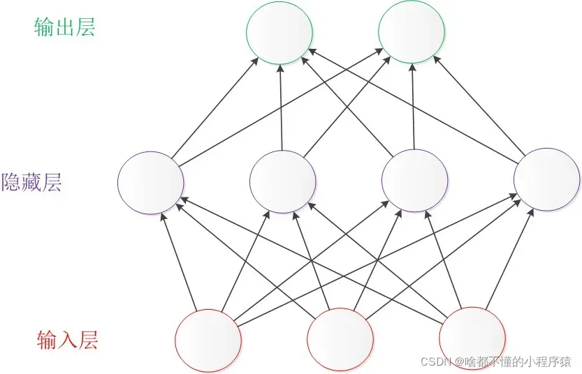
至于比较简单的神经网络,这里就简单说一下,让大家对神经网络有更深入的了解。先看下图,简单了解下。从下往上依次是输入层(输入数据)、隐藏层(包含数据信息)、输出层(输出结果)。奥秘也在隐藏层。通俗的讲,我们可以把这个网络看成一家公司。顶层是输出层是公司的最高管理层,隐藏层是公司的管理者,输入层是我们的员工。首先,员工负责收集数据并将其报告给经理。 ,并且每个经理会因为他不同的工作范围和偏好而偏好不同的输入层。比如最左边的隐藏层更喜欢输入层左边第一个和第三个员工的输入,而第二个第二个和第四个员工的输入不是很敏感,所以当第一个员工输入的数据时而第三个员工到了,隐藏层的经理立即了解并发现其中包含的信息,然后通知上级即输出层的上层。输出层的第一个顶层也对第一个隐藏层的管理器和第四个隐藏层的管理器敏感。第一个顶层根据隐藏层的第一个管理器和第四个管理器提供的信息做出决策。 .这代表输出。不过有一点需要注意,因为神经网络是全连接的,所以对于第一个隐藏层的经理来说,他其实和所有员工都有联系,四个员工中只有一个员工和第三个员工。每个员工都比较敏感,或者关系比较高。这样,随着时间的推移,它们的关系越来越好,而且彼此之间也非常敏感,这样基本上我们就可以大致了解收集数据信息的神经网络全连接隐藏层和输出层的奥秘了根据数据信息做出决策。
1.2 理论分析
1.2.1 BP神经网络的基本结构
最基本的神经网络由输入层、输出层和隐藏层组成。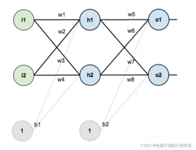
1.2.2 BP神经网络的重点——反向传播
反向传播的核心是高等数学中的链式法则推导。反向传播有两个主要步骤:
(1) 计算总误差
(2) 隐含层到输出层的权值更新(利用整体误差对某个权值求偏导运用链式法则)
具体计算如图,用
如果神经网络的层数很大,会导致导数很多,而神经网络的误差传播算法就是用序列的递推关系代替复杂的导数计算。更准确地说,误差是从后到前逐层计算和更新的权重。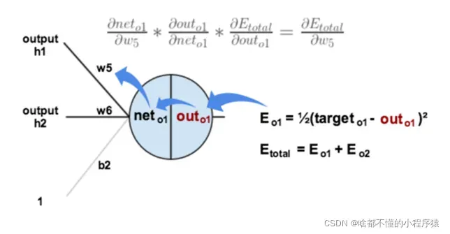
1.2.3 BP神经网络主要过程
神经网络主要流程概述
BP神经网络是一种非线性多层前向反馈网络,也就是多了一个反向传播的过程。基本思路就是,模型每进行一次前向传播之后,计算输出层与目标函数之间的误差,再将结果代入激活函数的导数计算之后,返回给离输出层最近的隐层,再计算当前隐层与上一层之间的误差,然后逐渐往回传播,直到第一个隐层为止。进行一次反向传播之后,还需要对权重参数进行更新。
神经网络的具体操作
(1) 初始化参数
(2) 构造损失函数Loss函数(①交叉熵②平方法)
(3) 正向传导→(
(4) 结束条件:(①
(5) 根据梯度下降(GD)来←反向传播(目的是更新权重)
二、代码实现
这是我们使用传统代码实现的一个案例。
假设,你有这样一个网络层: 第一层是输入层,包含两个神经元 i1,i2,和截距项 b1;第二层是隐含层, 包含两个神经元 h1,h2 和截距项 b2,第三层是输出 o1,o2,每条线上标的 wi 是层与层之间连接的权重,激活函数我们默认为 sigmoid 函数。现在对他们赋上初值,如下图:
目标:给出输入数据 i1,i2(0.05 和 0.10),使输出尽可能与原始输出 o1,o2(0.01 和 0.99)接近。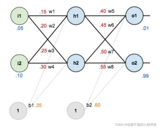
# !/usr/bin/env python
# @Time:2022/3/26 15:54
# @Author:华阳
# @File:ANN.py
# @Software:PyCharm
# 参数解释:
# "pd_" :偏导的前缀
# "d_" :导数的前缀
# "w_ho" :隐含层到输出层的权重系数索引
# "w_ih" :输入层到隐含层的权重系数的索引
import math
import matplotlib.pyplot as plt
class NeuralNetwork:
LEARNING_RATE = 0.5
def __init__(self, num_inputs, num_hidden, num_outputs, hidden_layer_weights=None, hidden_layer_bias=None,
output_layer_weights=None, output_layer_bias=None):
self.num_inputs = num_inputs
self.hidden_layer = NeuronLayer(num_hidden, hidden_layer_bias)
self.output_layer = NeuronLayer(num_outputs, output_layer_bias)
self.init_weights_from_inputs_to_hidden_layer_neurons(hidden_layer_weights)
self.init_weights_from_hidden_layer_neurons_to_output_layer_neurons(output_layer_weights)
def init_weights_from_inputs_to_hidden_layer_neurons(self, hidden_layer_weights):
weight_num = 0
for h in range(len(self.hidden_layer.neurons)):
for i in range(self.num_inputs):
if not hidden_layer_weights:
self.hidden_layer.neurons[h].weights.append(random.random())
else:
self.hidden_layer.neurons[h].weights.append(hidden_layer_weights[weight_num])
weight_num += 1
def init_weights_from_hidden_layer_neurons_to_output_layer_neurons(self, output_layer_weights):
weight_num = 0
for o in range(len(self.output_layer.neurons)):
for h in range(len(self.hidden_layer.neurons)):
if not output_layer_weights:
self.output_layer.neurons[o].weights.append(random.random())
else:
self.output_layer.neurons[o].weights.append(output_layer_weights[weight_num])
weight_num += 1
def inspect(self):
print('------')
print('* Inputs: {}'.format(self.num_inputs))
print('------')
print('Hidden Layer')
self.hidden_layer.inspect()
print('------')
print('* Output Layer')
self.output_layer.inspect()
print('------')
def feed_forward(self, inputs):
hidden_layer_outputs = self.hidden_layer.feed_forward(inputs)
return self.output_layer.feed_forward(hidden_layer_outputs)
def train(self, training_inputs, training_outputs):
self.feed_forward(training_inputs)
# 1. 输出神经元的值
pd_errors_wrt_output_neuron_total_net_input = [0] * len(self.output_layer.neurons)
for o in range(len(self.output_layer.neurons)):
# ∂E/∂zⱼ
pd_errors_wrt_output_neuron_total_net_input[o] = self.output_layer.neurons[
o].calculate_pd_error_wrt_total_net_input(training_outputs[o])
# 2. 隐含层神经元的值
pd_errors_wrt_hidden_neuron_total_net_input = [0] * len(self.hidden_layer.neurons)
for h in range(len(self.hidden_layer.neurons)):
# dE/dyⱼ = Σ ∂E/∂zⱼ * ∂z/∂yⱼ = Σ ∂E/∂zⱼ * wᵢⱼ
d_error_wrt_hidden_neuron_output = 0
for o in range(len(self.output_layer.neurons)):
d_error_wrt_hidden_neuron_output += pd_errors_wrt_output_neuron_total_net_input[o] * \
self.output_layer.neurons[o].weights[h]
# ∂E/∂zⱼ = dE/dyⱼ * ∂zⱼ/∂
pd_errors_wrt_hidden_neuron_total_net_input[h] = d_error_wrt_hidden_neuron_output * \
self.hidden_layer.neurons[
h].calculate_pd_total_net_input_wrt_input()
# 3. 更新输出层权重系数
for o in range(len(self.output_layer.neurons)):
for w_ho in range(len(self.output_layer.neurons[o].weights)):
# ∂Eⱼ/∂wᵢⱼ = ∂E/∂zⱼ * ∂zⱼ/∂wᵢⱼ
pd_error_wrt_weight = pd_errors_wrt_output_neuron_total_net_input[o] * self.output_layer.neurons[
o].calculate_pd_total_net_input_wrt_weight(w_ho)
# Δw = α * ∂Eⱼ/∂wᵢ
self.output_layer.neurons[o].weights[w_ho] -= self.LEARNING_RATE * pd_error_wrt_weight
# 4. 更新隐含层的权重系数
for h in range(len(self.hidden_layer.neurons)):
for w_ih in range(len(self.hidden_layer.neurons[h].weights)):
# ∂Eⱼ/∂wᵢ = ∂E/∂zⱼ * ∂zⱼ/∂wᵢ
pd_error_wrt_weight = pd_errors_wrt_hidden_neuron_total_net_input[h] * self.hidden_layer.neurons[
h].calculate_pd_total_net_input_wrt_weight(w_ih)
# Δw = α * ∂Eⱼ/∂wᵢ
self.hidden_layer.neurons[h].weights[w_ih] -= self.LEARNING_RATE * pd_error_wrt_weight
def calculate_total_error(self, training_sets):
total_error = 0
for t in range(len(training_sets)):
training_inputs, training_outputs = training_sets[t]
self.feed_forward(training_inputs)
for o in range(len(training_outputs)):
total_error += self.output_layer.neurons[o].calculate_error(training_outputs[o])
return total_error
class NeuronLayer:
def __init__(self, num_neurons, bias):
# 同一层的神经元共享一个截距项 b
self.bias = bias if bias else random.random()
self.neurons = []
for i in range(num_neurons):
self.neurons.append(Neuron(self.bias))
def inspect(self):
print('Neurons:', len(self.neurons))
for n in range(len(self.neurons)):
print(' Neuron', n)
for w in range(len(self.neurons[n].weights)):
print(' Weight:', self.neurons[n].weights[w])
print(' Bias:', self.bias)
def feed_forward(self, inputs):
outputs = []
for neuron in self.neurons:
outputs.append(neuron.calculate_output(inputs))
return outputs
def get_outputs(self):
outputs = []
for neuron in self.neurons:
outputs.append(neuron.output)
return outputs
class Neuron:
def __init__(self, bias):
self.bias = bias
self.weights = []
def calculate_output(self, inputs):
self.inputs = inputs
self.output = self.squash(self.calculate_total_net_input())
return self.output
def calculate_total_net_input(self):
total = 0
for i in range(len(self.inputs)):
total += self.inputs[i] * self.weights[i]
return total + self.bias
# 激活函数 sigmoid
def squash(self, total_net_input):
return 1 / (1 + math.exp(-total_net_input))
def calculate_pd_error_wrt_total_net_input(self, target_output):
return self.calculate_pd_error_wrt_output(target_output) * self.calculate_pd_total_net_input_wrt_input();
# 每一个神经元的误差是由平方差公式计算的
def calculate_error(self, target_output):
return 0.5 * (target_output - self.output) ** 2
def calculate_pd_error_wrt_output(self, target_output):
return -(target_output - self.output)
def calculate_pd_total_net_input_wrt_input(self):
return self.output * (1 - self.output)
def calculate_pd_total_net_input_wrt_weight(self, index):
return self.inputs[index]
# 文中的例子:
nn = NeuralNetwork(2, 2, 2, hidden_layer_weights=[0.15, 0.2, 0.25, 0.3], hidden_layer_bias=0.35,
output_layer_weights=[0.4, 0.45, 0.5, 0.55], output_layer_bias=0.6)
losses = []
for i in range(1000):
nn.train([0.05, 0.1], [0.01, 0.09])
losses.append(round(nn.calculate_total_error([[[0.05, 0.1], [0.01, 0.09]]]), 9))
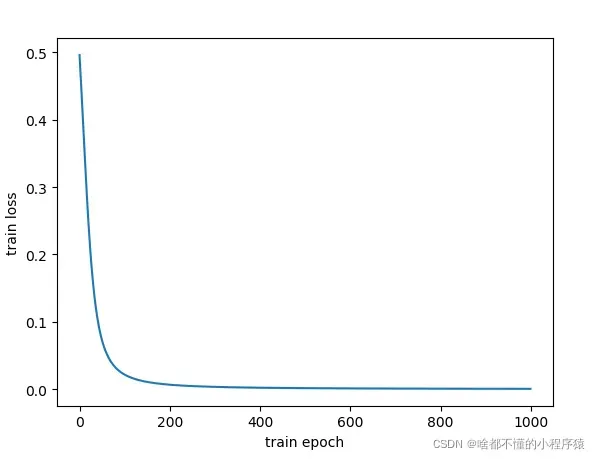
plt.plot(losses)
plt.xlabel("train epoch")
plt.ylabel("train loss")
plt.show()
nn.inspect()
运行代码的结果:
------
* Inputs: 2
------
Hidden Layer
Neurons: 2
 Neuron 0
 Weight: 0.2964604103620042
 Weight: 0.49292082072400834
 Bias: 0.35
 Neuron 1
 Weight: 0.39084333156627366
 Weight: 0.5816866631325477
 Bias: 0.35
------
* Output Layer
Neurons: 2
 Neuron 0
 Weight: -3.060957226462873
 Weight: -3.0308626603447846
 Bias: 0.6
 Neuron 1
 Weight: -2.393475400842236
 Weight: -2.3602088337272704
 Bias: 0.6
------
看到上面的结果你是不是想到了放弃,哈哈,没必要的这样。这样确实对于搞AI的太难了,所以大佬们都把复杂的训练的与构造过程集成化,编写了一系列的框架,最常用的以pytorch,paddlepaddle,keras,tensorflow。其中个人认为keras,对新手比较友好。可以用于入门构造网络,但是更深层里的框架还是其他三种更加适合。而keras需要由其他框架比如tensorflow作为后台。
大家可以用按住win+R键,打开运行窗口,输入cmd。
输入cmd,回车后,会显示如下。
输入以下的命令,可以看看自己的电脑的显卡是不是NVIDIA。如果是AMD的,那么就安装cpu的吧,毕竟CUDA内核,只支持NVIDIA的显卡。
#AMD显卡
pip install tensorflow-cpu
#NVIDIA显卡
pip install tensorflow
#有了后台以后就安装keras喽
pip install keras
#如果速度慢的话,可以加入清华源的链接
pip install tensorflow-cpu -i https://pypi.tuna.tsinghua.edu.cn/simple/
#NVIDIA显卡
pip install tensorflow -i https://pypi.tuna.tsinghua.edu.cn/simple/
#有了后台以后就安装keras喽
pip install keras -i https://pypi.tuna.tsinghua.edu.cn/simple/
利用keras构建MLP进行二分类:印第安人糖尿病预测
# 2.1 引入相关模块
import warnings
warnings.filterwarnings("ignore")
import pandas as pd
import matplotlib.pyplot as plt
from sklearn.model_selection import train_test_split
from keras.models import Sequential
from keras.layers import Dense

# 2.2 准备数据
df = pd.read_csv('pima_data.csv', header=None)
data = df.values
X = data[:, :-1]
y = data[:, -1]
from sklearn.preprocessing import MinMaxScaler

scaler = MinMaxScaler()
scaler.fit(X)
X = scaler.transform(X)
X_train, X_test, y_train, y_test = train_test_split(X, y, test_size=0.3, random_state=4)
# 2.3 构建网络模型:定义输入层、隐含层、输出层神经元个数,采用的激活函数
model = Sequential()
model.add(Dense(12, input_dim=8, activation='relu'))
model.add(Dense(8, activation='relu'))
model.add(Dense(1, activation='sigmoid'))
model.summary()

# 2.4 编译模型:确定损失函数,优化器,以及评估指标
model.compile(loss='binary_crossentropy', optimizer='adam', metrics=['accuracy'])
# 2.5 训练模型:确定迭代的次数,批尺寸,是否显示训练过程
model.fit(X_train, y_train, epochs=100, batch_size=20, verbose=True)
# 2.6 评估模型
score = model.evaluate(X_test,y_test,verbose=False)
print("准确率为:{:.2f}%".format(score[1]*100))
运行结果:
Model: "sequential"
_________________________________________________________________
 Layer (type)                Output Shape              Param #
=================================================================
 dense (Dense)               (None, 12)                108

 dense_1 (Dense)             (None, 8)                 104

 dense_2 (Dense)             (None, 1)                 9

=================================================================
Total params: 221
Trainable params: 221
Non-trainable params: 0
_________________________________________________________________
Epoch 1/100
27/27 [==============================] - 1s 2ms/step - loss: 0.6956 - accuracy: 0.5102
Epoch 2/100
27/27 [==============================] - 0s 2ms/step - loss: 0.6832 - accuracy: 0.6499
Epoch 3/100
27/27 [==============================] - 0s 2ms/step - loss: 0.6765 - accuracy: 0.6499
Epoch 4/100
27/27 [==============================] - 0s 2ms/step - loss: 0.6709 - accuracy: 0.6480
Epoch 5/100
27/27 [==============================] - 0s 2ms/step - loss: 0.6660 - accuracy: 0.6480
Epoch 6/100
27/27 [==============================] - 0s 2ms/step - loss: 0.6611 - accuracy: 0.6480
Epoch 7/100
27/27 [==============================] - 0s 2ms/step - loss: 0.6569 - accuracy: 0.6480
Epoch 8/100
27/27 [==============================] - 0s 2ms/step - loss: 0.6534 - accuracy: 0.6480
Epoch 9/100
27/27 [==============================] - 0s 2ms/step - loss: 0.6499 - accuracy: 0.6480
Epoch 10/100
27/27 [==============================] - 0s 2ms/step - loss: 0.6468 - accuracy: 0.6480
Epoch 11/100
27/27 [==============================] - 0s 2ms/step - loss: 0.6431 - accuracy: 0.6499
Epoch 12/100
27/27 [==============================] - 0s 2ms/step - loss: 0.6394 - accuracy: 0.6480
Epoch 13/100
27/27 [==============================] - 0s 2ms/step - loss: 0.6361 - accuracy: 0.6555
Epoch 14/100
27/27 [==============================] - 0s 2ms/step - loss: 0.6322 - accuracy: 0.6536
Epoch 15/100
27/27 [==============================] - 0s 2ms/step - loss: 0.6278 - accuracy: 0.6611
Epoch 16/100
27/27 [==============================] - 0s 2ms/step - loss: 0.6220 - accuracy: 0.6574
Epoch 17/100
27/27 [==============================] - 0s 2ms/step - loss: 0.6162 - accuracy: 0.6723
Epoch 18/100
27/27 [==============================] - 0s 2ms/step - loss: 0.6103 - accuracy: 0.6723
Epoch 19/100
27/27 [==============================] - 0s 2ms/step - loss: 0.6063 - accuracy: 0.6760
Epoch 20/100
27/27 [==============================] - 0s 2ms/step - loss: 0.6028 - accuracy: 0.6760
Epoch 21/100
27/27 [==============================] - 0s 2ms/step - loss: 0.5982 - accuracy: 0.6667
Epoch 22/100
27/27 [==============================] - 0s 2ms/step - loss: 0.5939 - accuracy: 0.6741
Epoch 23/100
27/27 [==============================] - 0s 2ms/step - loss: 0.5891 - accuracy: 0.6834
Epoch 24/100
27/27 [==============================] - 0s 2ms/step - loss: 0.5854 - accuracy: 0.6834
Epoch 25/100
27/27 [==============================] - 0s 2ms/step - loss: 0.5814 - accuracy: 0.6872
Epoch 26/100
27/27 [==============================] - 0s 2ms/step - loss: 0.5793 - accuracy: 0.6853
Epoch 27/100
27/27 [==============================] - 0s 2ms/step - loss: 0.5752 - accuracy: 0.6872
Epoch 28/100
27/27 [==============================] - 0s 2ms/step - loss: 0.5716 - accuracy: 0.6927
Epoch 29/100
27/27 [==============================] - 0s 2ms/step - loss: 0.5666 - accuracy: 0.7020
Epoch 30/100
27/27 [==============================] - 0s 2ms/step - loss: 0.5642 - accuracy: 0.6927
Epoch 31/100
27/27 [==============================] - 0s 2ms/step - loss: 0.5610 - accuracy: 0.6927
Epoch 32/100
27/27 [==============================] - 0s 2ms/step - loss: 0.5565 - accuracy: 0.7002
Epoch 33/100
27/27 [==============================] - 0s 2ms/step - loss: 0.5534 - accuracy: 0.7002
Epoch 34/100
27/27 [==============================] - 0s 2ms/step - loss: 0.5510 - accuracy: 0.7132
Epoch 35/100
27/27 [==============================] - 0s 2ms/step - loss: 0.5463 - accuracy: 0.7244
Epoch 36/100
27/27 [==============================] - 0s 2ms/step - loss: 0.5439 - accuracy: 0.7151
Epoch 37/100
27/27 [==============================] - 0s 2ms/step - loss: 0.5412 - accuracy: 0.7095
Epoch 38/100
27/27 [==============================] - 0s 2ms/step - loss: 0.5370 - accuracy: 0.7151
Epoch 39/100
27/27 [==============================] - 0s 2ms/step - loss: 0.5327 - accuracy: 0.7207
Epoch 40/100
27/27 [==============================] - 0s 2ms/step - loss: 0.5297 - accuracy: 0.7356
Epoch 41/100
27/27 [==============================] - 0s 2ms/step - loss: 0.5269 - accuracy: 0.7225
Epoch 42/100
27/27 [==============================] - 0s 2ms/step - loss: 0.5233 - accuracy: 0.7300
Epoch 43/100
27/27 [==============================] - 0s 2ms/step - loss: 0.5193 - accuracy: 0.7374
Epoch 44/100
27/27 [==============================] - 0s 2ms/step - loss: 0.5172 - accuracy: 0.7318
Epoch 45/100
27/27 [==============================] - 0s 2ms/step - loss: 0.5143 - accuracy: 0.7505
Epoch 46/100
27/27 [==============================] - 0s 2ms/step - loss: 0.5087 - accuracy: 0.7523
Epoch 47/100
27/27 [==============================] - 0s 2ms/step - loss: 0.5064 - accuracy: 0.7449
Epoch 48/100
27/27 [==============================] - 0s 2ms/step - loss: 0.5031 - accuracy: 0.7467
Epoch 49/100
27/27 [==============================] - 0s 2ms/step - loss: 0.5013 - accuracy: 0.7561
Epoch 50/100
27/27 [==============================] - 0s 2ms/step - loss: 0.4979 - accuracy: 0.7393
Epoch 51/100
27/27 [==============================] - 0s 2ms/step - loss: 0.4953 - accuracy: 0.7523
Epoch 52/100
27/27 [==============================] - 0s 2ms/step - loss: 0.4918 - accuracy: 0.7542
Epoch 53/100
27/27 [==============================] - 0s 2ms/step - loss: 0.4907 - accuracy: 0.7635
Epoch 54/100
27/27 [==============================] - 0s 2ms/step - loss: 0.4864 - accuracy: 0.7598
Epoch 55/100
27/27 [==============================] - 0s 2ms/step - loss: 0.4850 - accuracy: 0.7542
Epoch 56/100
27/27 [==============================] - 0s 2ms/step - loss: 0.4837 - accuracy: 0.7654
Epoch 57/100
27/27 [==============================] - 0s 2ms/step - loss: 0.4800 - accuracy: 0.7579
Epoch 58/100
27/27 [==============================] - 0s 2ms/step - loss: 0.4779 - accuracy: 0.7598
Epoch 59/100
27/27 [==============================] - 0s 2ms/step - loss: 0.4778 - accuracy: 0.7635
Epoch 60/100
27/27 [==============================] - 0s 2ms/step - loss: 0.4749 - accuracy: 0.7579
Epoch 61/100
27/27 [==============================] - 0s 2ms/step - loss: 0.4734 - accuracy: 0.7691
Epoch 62/100
27/27 [==============================] - 0s 2ms/step - loss: 0.4711 - accuracy: 0.7709
Epoch 63/100
27/27 [==============================] - 0s 2ms/step - loss: 0.4708 - accuracy: 0.7821
Epoch 64/100
27/27 [==============================] - 0s 2ms/step - loss: 0.4694 - accuracy: 0.7691
Epoch 65/100
27/27 [==============================] - 0s 2ms/step - loss: 0.4668 - accuracy: 0.7691
Epoch 66/100
27/27 [==============================] - 0s 2ms/step - loss: 0.4668 - accuracy: 0.7728
Epoch 67/100
27/27 [==============================] - 0s 2ms/step - loss: 0.4676 - accuracy: 0.7691
Epoch 68/100
27/27 [==============================] - 0s 2ms/step - loss: 0.4669 - accuracy: 0.7709
Epoch 69/100
27/27 [==============================] - 0s 2ms/step - loss: 0.4622 - accuracy: 0.7803
Epoch 70/100
27/27 [==============================] - 0s 2ms/step - loss: 0.4619 - accuracy: 0.7765
Epoch 71/100
27/27 [==============================] - 0s 2ms/step - loss: 0.4595 - accuracy: 0.7784
Epoch 72/100
27/27 [==============================] - 0s 2ms/step - loss: 0.4585 - accuracy: 0.7858
Epoch 73/100
27/27 [==============================] - 0s 2ms/step - loss: 0.4585 - accuracy: 0.7803
Epoch 74/100
27/27 [==============================] - 0s 2ms/step - loss: 0.4592 - accuracy: 0.7858
Epoch 75/100
27/27 [==============================] - 0s 2ms/step - loss: 0.4561 - accuracy: 0.7877
Epoch 76/100
27/27 [==============================] - 0s 2ms/step - loss: 0.4575 - accuracy: 0.7877
Epoch 77/100
27/27 [==============================] - 0s 2ms/step - loss: 0.4571 - accuracy: 0.7877
Epoch 78/100
27/27 [==============================] - 0s 2ms/step - loss: 0.4532 - accuracy: 0.7896
Epoch 79/100
27/27 [==============================] - 0s 2ms/step - loss: 0.4583 - accuracy: 0.7840
Epoch 80/100
27/27 [==============================] - 0s 2ms/step - loss: 0.4520 - accuracy: 0.7952
Epoch 81/100
27/27 [==============================] - 0s 2ms/step - loss: 0.4520 - accuracy: 0.7914
Epoch 82/100
27/27 [==============================] - 0s 2ms/step - loss: 0.4514 - accuracy: 0.7877
Epoch 83/100
27/27 [==============================] - 0s 2ms/step - loss: 0.4552 - accuracy: 0.7840
Epoch 84/100
27/27 [==============================] - 0s 2ms/step - loss: 0.4516 - accuracy: 0.7840
Epoch 85/100
27/27 [==============================] - 0s 2ms/step - loss: 0.4559 - accuracy: 0.7858
Epoch 86/100
27/27 [==============================] - 0s 2ms/step - loss: 0.4493 - accuracy: 0.7896
Epoch 87/100
27/27 [==============================] - 0s 2ms/step - loss: 0.4498 - accuracy: 0.7914
Epoch 88/100
27/27 [==============================] - 0s 2ms/step - loss: 0.4501 - accuracy: 0.7952
Epoch 89/100
27/27 [==============================] - 0s 2ms/step - loss: 0.4470 - accuracy: 0.7970
Epoch 90/100
27/27 [==============================] - 0s 2ms/step - loss: 0.4489 - accuracy: 0.7858
Epoch 91/100
27/27 [==============================] - 0s 2ms/step - loss: 0.4470 - accuracy: 0.8007
Epoch 92/100
27/27 [==============================] - 0s 2ms/step - loss: 0.4480 - accuracy: 0.8063
Epoch 93/100
27/27 [==============================] - 0s 2ms/step - loss: 0.4463 - accuracy: 0.8007
Epoch 94/100
27/27 [==============================] - 0s 3ms/step - loss: 0.4460 - accuracy: 0.7914
Epoch 95/100
27/27 [==============================] - 0s 2ms/step - loss: 0.4457 - accuracy: 0.7914
Epoch 96/100
27/27 [==============================] - 0s 2ms/step - loss: 0.4469 - accuracy: 0.7989
Epoch 97/100
27/27 [==============================] - 0s 2ms/step - loss: 0.4451 - accuracy: 0.8007
Epoch 98/100
27/27 [==============================] - 0s 2ms/step - loss: 0.4438 - accuracy: 0.7989
Epoch 99/100
27/27 [==============================] - 0s 2ms/step - loss: 0.4435 - accuracy: 0.8026
Epoch 100/100
27/27 [==============================] - 0s 2ms/step - loss: 0.4434 - accuracy: 0.8026
准确率为:75.76%

Process finished with exit code 0
文章出处登录后可见!