学习目标：

机器学习分类模型的评估

学习内容：

了解如何评估分类模型：
1、混淆矩阵
2、分类结果汇总
3、ROC曲线
4、召回率与精度
5、F1分数

基础知识：

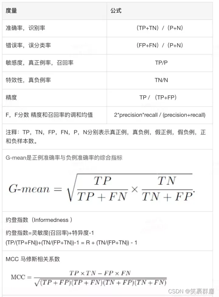
1. 评估分类器性能的指标
1、真正(true positive, TP)或f++，对应的是被分类模型正确预测的正样本数。
2、假负(false negative, FN)或f±对应的是被分类模型错误预测为负类的正样本数。
3、假正(false positive, FP)或f-+, .对应的是被分类模型错误预测为正类的负样本数。
4、真负(ture negative, TN)或f–， 对应的是被分类模型正确预测的负样本数。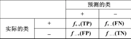

实验步骤：

1. 混淆矩阵

1、导入鸢尾花数据集

from sklearn.datasets import load_iris
iris = load_iris()

2、二分法拆分数据

from sklearn.model_selection import train_test_split
x_train,x_test,y_train,y_test = train_test_split(iris.data,iris.target,test_size = 0.3,random_state = 666)

3、构建决策树模型

from sklearn.tree import DecisionTreeClassifier
dt = DecisionTreeClassifier()
dt.fit(x_train, y_train)

结果是：

DecisionTreeClassifier()

4、模型预测

dt.predict(x_test)

结果是：

array([1, 2, 1, 2, 0, 1, 1, 2, 1, 1, 1, 0, 0, 0, 2, 1, 0, 2, 2, 2, 1, 0,
       2, 0, 1, 1, 0, 1, 2, 2, 0, 0, 1, 2, 1, 1, 2, 2, 0, 1, 2, 2, 1, 1,
       0])

5、模型评估

from sklearn.metrics import classification_report#导入混淆矩阵对应的库
print(classification_report(y_test,dt.predict(x_test)))

结果是：

                precision    recall  f1-score   support

           0       1.00      1.00      1.00        12
           1       1.00      1.00      1.00        18
           2       1.00      1.00      1.00        15

    accuracy                           1.00        45
   macro avg       1.00      1.00      1.00        45
weighted avg       1.00      1.00      1.00        45

6、输出训练集上的混淆矩阵

#混淆矩阵
from sklearn.metrics import confusion_matrix
cm = confusion_matrix(y_train,dt.predict(x_train))
cm

结果是：

array([[38,  0,  0],
       [ 0, 32,  0],
       [ 0,  0, 35]], dtype=int64)

#自定义类别顺序输出混淆矩阵
confusion_matrix(y_train,dt.predict(x_train),labels = [2,1,0])

结果是：

array([[35,  0,  0],
       [ 0, 32,  0],
       [ 0,  0, 38]], dtype=int64)

7、用热力图展示混淆矩阵

#用热力图展示混淆矩阵
%matplotlib inline
import matplotlib.pyplot as plt
import seaborn as sns
sns.heatmap(cm,cmap = sns.color_palette("Blues"),annot = True)

结果如下：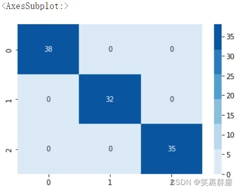

**【注意】：**在热力图中需要提前电脑安装matplotlib库，否则无法使用热力图
安装matplotlib库方法：打Anaconda => Anaconda Prompt => 输入 pip install matplotlib
等待安装完成。

**

两种分类结果总结

**

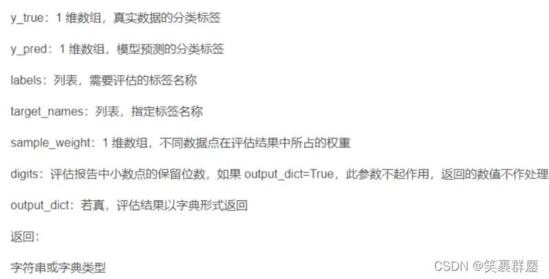
from sklearn.metrics import classification_report
a = classification_report(y_train,
                          dt.predict(x_train),
                          digits = 3,#小数点后保留的位数
                          labels = [2,1,0],#类别的排序
                          target_names = ['第2类','第1类','第0类'],#类别的名称
                          output_dict = False)#结果是否以字典的形式输出
print(a)

结果是：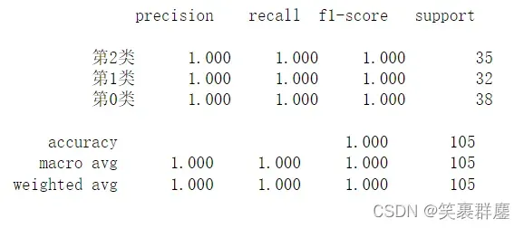

三、ROC曲线

1、导入所需要的库
数据集如下：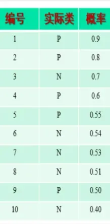

from sklearn.metrics import roc_curve
#录入数据
import numpy as np
y_true = np.array([1,1,0,1,1,0,0,0,1,0])
y_score = np.array([0.9,0.8,0.7,0.6,0.55,0.54,0.53,0.51,0.50,0.40])

2、调用roc_curve 求出fpr与tpr

fpr,tpr,thresholds = roc_curve(y_true,y_score)

3、打印结果

print(fpr,tpr,thresholds,sep = '\n')

结果是：

[0.  0.  0.  0.2 0.2 0.8 0.8 1. ]
[0.  0.2 0.4 0.4 0.8 0.8 1.  1. ]
[1.9  0.9  0.8  0.7  0.55 0.51 0.5  0.4 ]

4、修改参数drop_intermediate 值为False

fpr1,tpr1,thresholds1 = roc_curve(y_true,y_score,drop_intermediate = False)

输出结果：

print(fpr1,tpr1,thresholds1,sep = '\n')

结果：

[0.  0.  0.  0.2 0.2 0.2 0.4 0.6 0.8 0.8 1. ]
[0.  0.2 0.4 0.4 0.6 0.8 0.8 0.8 0.8 1.  1. ]
[1.9  0.9  0.8  0.7  0.6  0.55 0.54 0.53 0.51 0.5  0.4 ]

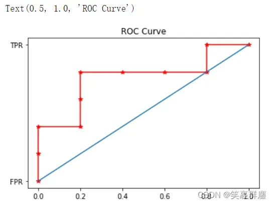
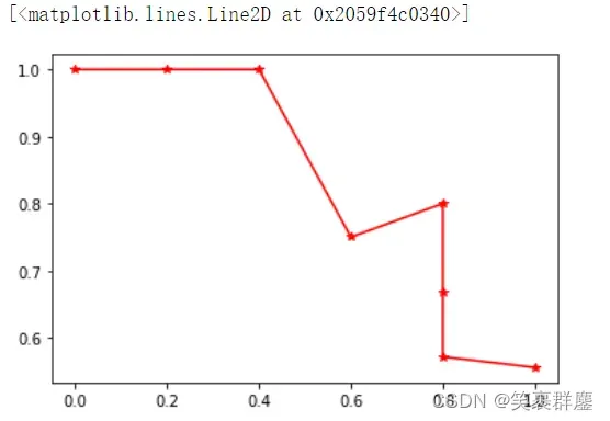
5、绘制ROC曲线

plt.plot(fpr1,tpr1,'r*-')
plt.plot([0,1],[0,1])
plt.plot("FPR")
plt.plot("TPR")
plt.title("ROC Curve")

6、计算ROC曲线下的面积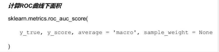

from sklearn.metrics import roc_auc_score
roc_auc_score(y_true,y_score)

结果是：

0.76

4.召回率和准确率

模型评价：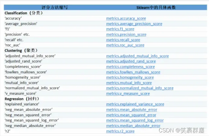

1、导入所需的库

import numpy as np
from sklearn.metrics import precision_recall_curve

2、录入数据

y_true = np.array([0,0,0,0,0,1,1,1,1,1])
y_scores = np.array([0.1,0.2,0.25,0.4,0.6,0.2,0.45,0.6,0.75,0.8])

3、召回率与精度的计算

precision,recall,thresholds = precision_recall_curve(y_true,y_scores)
len(precision),len(recall),len(thresholds)

结果是：

(8, 8, 7)

thresholds

结果是：

array([0.2 , 0.25, 0.4 , 0.45, 0.6 , 0.75, 0.8 ])

召回率：

precision

结果是：

array([0.55555556, 0.57142857, 0.66666667, 0.8       , 0.75      ,
       1.        , 1.        , 1.        ])

准确性：

recall

结果是：

array([1. , 0.8, 0.8, 0.8, 0.6, 0.4, 0.2, 0. ])

#plt.grid()

plt.scatter(thresholds,precision[:-1])

结果是：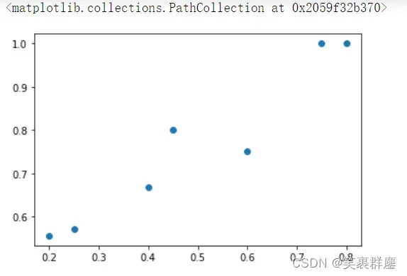

回忆散点图：

plt.scatter(thresholds,recall[:-1])

结果是：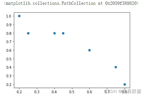

精度散点图：

plt.scatter(recall,precision)

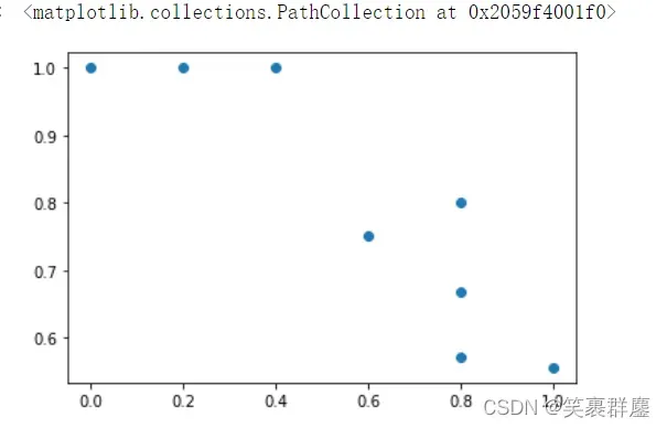
plt.plot(recall,precision,'r-*')

4、多值预测问题需要转化为二值预测问题进行评估

from sklearn.preprocessing import binarize
y = binarize(iris.target.reshape(-1,1))

5、输出预测的平均精确率

from sklearn.metrics import average_precision_score
average_precision = average_precision_score(y_true,y_scores)
average_precision

结果是：

0.8211111111111111

*

五、F1分数

1、导入所需的库

from sklearn.metrics import f1_score
from sklearn.neural_network import MLPClassifier
mlp = MLPClassifier()
mlp.fit(iris.data,iris.target)

2、进行F1分数计算

f1_score(iris.target,mlp.predict(iris.data),average = 'micro')

0.9733333333333334

f1_score(iris.target,mlp.predict(iris.data),average = 'macro')

0.9732905982905983

f1_score(iris.target,mlp.predict(iris.data),average = 'weighted')

0.9732905982905984