1 问题描述

给定50个正弦函数的数据对（x, y），划分0~48（前49个）是训练数据集，（1~50）是预测数据集。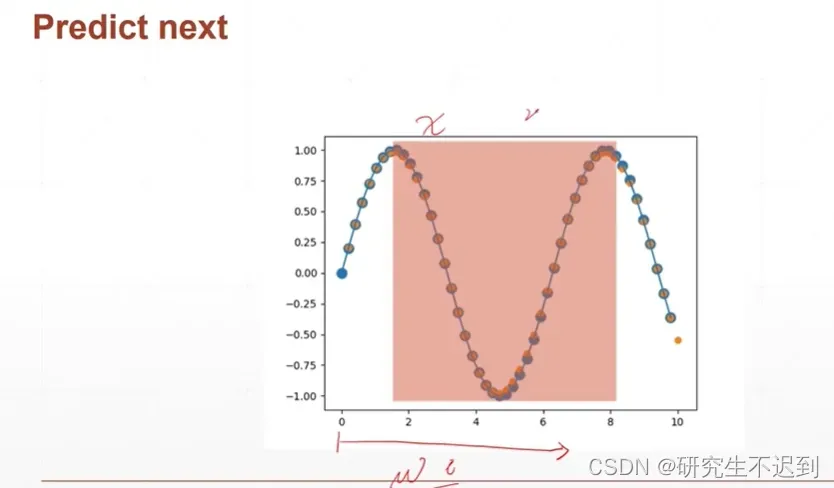

2 数据处理部分

	num_time_steps = 50 

    start = np.random.randint(3, size=1)[0]  # 返回[0,3)范围内的整数
    time_steps = np.linspace(start, start + 10, num_time_steps)
    data = np.sin(time_steps)
    data = data.reshape(num_time_steps, 1)
    x = torch.tensor(data[:-1]).float().view(1, num_time_steps - 1, 1)
    y = torch.tensor(data[1:]).float().view(1, num_time_steps - 1, 1)

2.1 np.random.randint()

函数原型

randint(low, high=None, size=None, dtype=None)

参数介绍

（1）low : int
表示生成的数值大于等于low。
但是如果hign = None时，生成的数值要在[0, low)区间内【代码中用的就是这一种，表示生成的是[0,3) 之间的一个整数】

（2）high : int (可选，默认None)
如果使用这个值，则生成的数值在[low, high)区间

（3）size : int or tuple of ints(可选)
输出随机数组的尺寸，比如size = (m, n, k)，则输出数组的shape = (m, n, k)，数组中的每个元素均满足要求。
size默认为None，仅仅返回满足要求的单一随机数。

（4）dtype : dtype(可选)：
想要输出的格式。如int64、int等等

2.2 np.linspace()

函数原型

linspace(start, stop, num=50, endpoint=True, retstep=False, dtype=None,
             axis=0):

参数介绍：

（1）start : 返回样本数据开始点
（2）stop : 返回样本数据结束点
（3）num : 生成的样本数据量，默认为50
（4）endpoint：True则包含stop；False则不包含stop
（5）retstep：If True, return (samples, step), where step is the spacing between samples.(即如果为True则结果会给出数据间隔)
（6）dtype：输出数组类型
（7）axis：0(默认)或-1

在代码中， time_steps = np.linspace(start, start + 10, num_time_steps) 表示在[start , start+10)中等距生成50个点。

例如：

time = np.linspace(3, 13, 50)
time
array([ 3.        ,  3.20408163,  3.40816327,  3.6122449 ,  3.81632653,
        4.02040816,  4.2244898 ,  4.42857143,  4.63265306,  4.83673469,
        5.04081633,  5.24489796,  5.44897959,  5.65306122,  5.85714286,
        6.06122449,  6.26530612,  6.46938776,  6.67346939,  6.87755102,
        7.08163265,  7.28571429,  7.48979592,  7.69387755,  7.89795918,
        8.10204082,  8.30612245,  8.51020408,  8.71428571,  8.91836735,
        9.12244898,  9.32653061,  9.53061224,  9.73469388,  9.93877551,
       10.14285714, 10.34693878, 10.55102041, 10.75510204, 10.95918367,
       11.16326531, 11.36734694, 11.57142857, 11.7755102 , 11.97959184,
       12.18367347, 12.3877551 , 12.59183673, 12.79591837, 13.        ])

2.3 最终的数据情况

data.shape : 50 × 1
x的数据内容是data的 0~48（共计49个数）， y的数据内容化是data 的1~ 49（共计49个数）， (x, y)是一组数据对，是相邻的两个数据。
最后reshape了 x和y ，shape 是 [1, 49, 1]，再把np类型的数据转换为torch.tensor 这样才能喂给模型。

3 模型介绍

在看这一部分内容，一定要有RNN的基础知识，比如说输出数据的 shape，中间memory 的shape 和最后输出的数据的shape 之间的关系，如果不清楚的话，可以看我同系列的时间序列学习（1~3）

3.1 模型代码

input_size = 1
hidden_size = 16
output_size = 1

class Net(nn.Module):

    def __init__(self, ):
        super(Net, self).__init__()
        self.rnn = nn.RNN(input_size=input_size, hidden_size=hidden_size, num_layers=1, batch_first=True)
        self.linear = nn.Linear(in_features=hidden_size, out_features=output_size)


    def forward(self, x, hidden_prev):

       out, hidden_prev = self.rnn(x, hidden_prev)
       # [b, seq, h]
       out = out.view(-1, hidden_size)
       out = self.linear(out)
       out = out.unsqueeze(dim=0)
       return out, hidden_prev

3.2 介绍 init 函数

init 函数中，定义了两个层，一个是 rnn 一个是linear

对于rnn层，看参数中的 batch_first=True ，说明这里喂给rnn 的数据应该是：[batch , seq, feature] （就是把batch提前，因为batch_first = True 嘛）
然后就是 input_size=input_size=1 ，表示输入的数据的特征维度，因为这里就是数字数据，所以feature=1（不需要像词向量处理一样，把词转换成100d 的向量了）
对于hidden_size ，就是自己可以指定数据在处理中的特征维度，比如说16， 20等等都是可以的，这里选择16
num_layers=1 表示rnn 只有一层

对于linear层，in_features=hidden_size 表示输入数据的特征维度，out_features=output_size 表示输出数据的特征维度

3.3 介绍forward函数

该功能集成了模型的执行。

首先调用 self.rnn ，在调用时，需要传入两个参数，一个是训练数据x（x.shape = batch * seq * hidden_features）；另一个是，是一个在循环神经网络中的记忆单元，是会一直向后传播的。【可以不传入直接让 rnn 自己生成也可以】

out, hidden_prev = self.rnn(x, hidden_prev)

对于 self.rnn 的输出，out 和hidden_prev 的shape，是可以根据前面的已有信息计算出来的。如果觉得推理麻烦，也可以使用 torchsummary 直接查看。
out.shape : [1, 49, 16]
hidden.prev.shape : [1, 1, 16]

# 首先安装 torchsummary
pip intall torchsummary

# 然后在需要引用的地方，用下面语句调用
summary(model, input_size, batch_size=-1, device="cuda")
#这里是函数原型

4 模型训练部分

model = Net()
criterion = nn.MSELoss()
optimizer = optim.Adam(model.parameters(), lr)

hidden_prev = torch.zeros(1, 1, hidden_size)  # h0

for iter in range(1000):
    start = np.random.randint(3, size=1)[0]
    time_steps = np.linspace(start, start + 10, num_time_steps)
    data = np.sin(time_steps)
    data = data.reshape(num_time_steps, 1)
    x = torch.tensor(data[:-1]).float().view(1, num_time_steps - 1, 1)
    y = torch.tensor(data[1:]).float().view(1, num_time_steps - 1, 1)

    output, hidden_prev = model(x, hidden_prev)
    hidden_prev = hidden_prev.detach()

    loss = criterion(output, y)
    model.zero_grad()
    loss.backward()

    optimizer.step()

    if iter % 100 == 0:
        print("Iteration: {} loss {}".format(iter, loss.item()))

4.1 同数据处理部分

我不会详细介绍这一点。

    start = np.random.randint(3, size=1)[0]
    time_steps = np.linspace(start, start + 10, num_time_steps)
    data = np.sin(time_steps)
    data = data.reshape(num_time_steps, 1)
    x = torch.tensor(data[:-1]).float().view(1, num_time_steps - 1, 1)
    y = torch.tensor(data[1:]).float().view(1, num_time_steps - 1, 1)

4.2 喂数据给模型、计算loss、梯度更新，反向传播

传递给模型输入和初始
detach() 的作用是深拷贝

tensor.detach()是为了解决tensor.data()的安全性提出的。tensor.detach()相对较为安全。因为当通过.detach()得到的tensor间接修改原来的tensor后继续在计算图中使用时会报错，但是通过.data()得到的tensor间接修改原tensor后继续在计算图中使用就会被忽略被修改的过程

criterion是前面定义的函数，然后就是反向传播的固定写法。

    output, hidden_prev = model(x, hidden_prev)
    hidden_prev = hidden_prev.detach()

    loss = criterion(output, y)
    model.zero_grad()
    loss.backward()

    optimizer.step()

    if iter % 100 == 0:
        print("Iteration: {} loss {}".format(iter, loss.item()))

5 模型预测部分

5.1 同数据处理部分

这里的一个问题是训练集和预测集交叉，这是不好的。

start = np.random.randint(3, size=1)[0]
time_steps = np.linspace(start, start + 10, num_time_steps)
data = np.sin(time_steps)
data = data.reshape(num_time_steps, 1)
x = torch.tensor(data[:-1]).float().view(1, num_time_steps - 1, 1)
y = torch.tensor(data[1:]).float().view(1, num_time_steps - 1, 1)

predictions = []
input = x[:, 0, :]
for _ in range(x.shape[1]):
  input = input.view(1, 1, 1)
  (pred, hidden_prev) = model(input, hidden_prev)
  input = pred
  predictions.append(pred.detach().numpy().ravel()[0])

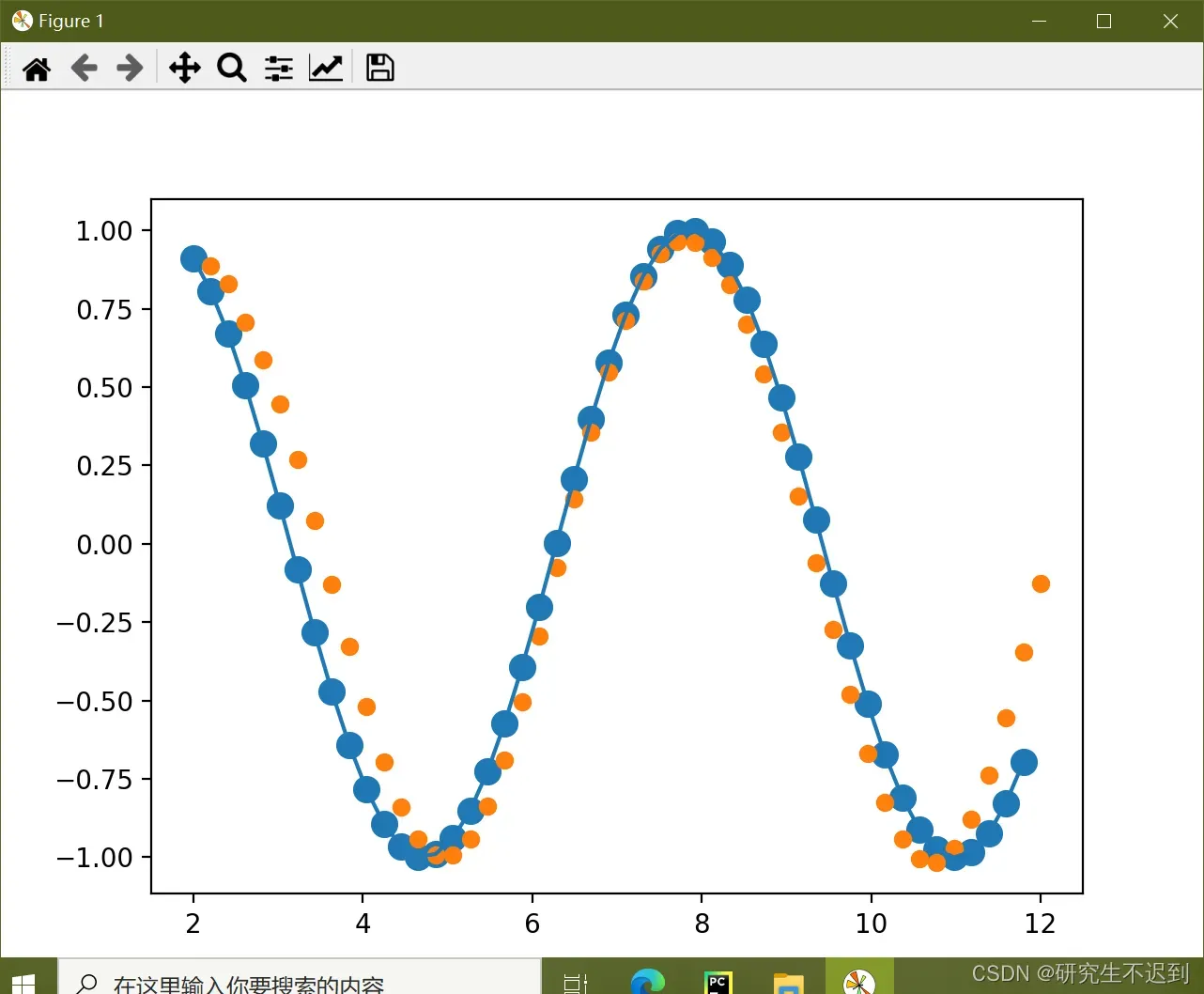
6 画图

x = x.data.numpy().ravel()
y = y.data.numpy()
plt.scatter(time_steps[:-1], x.ravel(), s=90)
plt.plot(time_steps[:-1], x.ravel())

plt.scatter(time_steps[1:], predictions)
plt.show()

7 完整代码，可以直接运行

如果你觉得对你有帮助，请点赞和关注我！你的支持是我分享的动力~


import numpy as np
import torch
from torch import nn, optim
import matplotlib.pyplot as plt
from torchsummary import summary
import os
os.environ["KMP_DUPLICATE_LIB_OK"] = "TRUE"


num_time_steps = 50
input_size = 1
hidden_size = 16
output_size = 1
lr = 0.01
hidden_prev = torch.zeros(1, 1, hidden_size)

class Net(nn.Module):
    def __init__(self, ):
        super(Net, self).__init__()
        self.rnn = nn.RNN(input_size=input_size, hidden_size=hidden_size, num_layers=1, batch_first=True)
        self.linear = nn.Linear(hidden_size, output_size)

    def forward(self, x, hidden_prev):
        out, hidden_prev = self.rnn(x, hidden_prev)
        # [b, seq, h]
        print(out.shape, hidden_prev.shape)
        out = out.view(-1, hidden_size)  # [1, seq, hidden] -> [seq, hidden]
        out = self.linear(out)  # [seq, hidden] -> [seq, 1]
        out = out.unsqueeze(dim=0)  # -> [1, seq, 1]  这里要和y做均方差
        return out, hidden_prev


model = Net()
criterion = nn.MSELoss()
optimizer = optim.Adam(model.parameters(), lr)

hidden_prev = torch.zeros(1, 1, hidden_size)  # h0

for iter in range(1000):
    start = np.random.randint(3, size=1)[0]
    time_steps = np.linspace(start, start + 10, num_time_steps)
    data = np.sin(time_steps)
    data = data.reshape(num_time_steps, 1)
    x = torch.tensor(data[:-1]).float().view(1, num_time_steps - 1, 1)
    y = torch.tensor(data[1:]).float().view(1, num_time_steps - 1, 1)

    output, hidden_prev = model(x, hidden_prev)
    hidden_prev = hidden_prev.detach()

    loss = criterion(output, y)
    model.zero_grad()
    loss.backward()

    optimizer.step()

    if iter % 100 == 0:
        print("Iteration: {} loss {}".format(iter, loss.item()))


start = np.random.randint(3, size=1)[0]
time_steps = np.linspace(start, start + 10, num_time_steps)
data = np.sin(time_steps)
data = data.reshape(num_time_steps, 1)
x = torch.tensor(data[:-1]).float().view(1, num_time_steps - 1, 1)
y = torch.tensor(data[1:]).float().view(1, num_time_steps - 1, 1)

predictions = []
input = x[:, 0, :]
for _ in range(x.shape[1]):
  input = input.view(1, 1, 1)
  (pred, hidden_prev) = model(input, hidden_prev)
  input = pred
  predictions.append(pred.detach().numpy().ravel()[0])

x = x.data.numpy().ravel()
y = y.data.numpy()
plt.scatter(time_steps[:-1], x.ravel(), s=90)
plt.plot(time_steps[:-1], x.ravel())

plt.scatter(time_steps[1:], predictions)
plt.show()

文章出处登录后可见！

已经登录？立即刷新

时间序列学习（4）——【正弦函数预测，RNN，代码+详解】非常清楚，强烈推荐