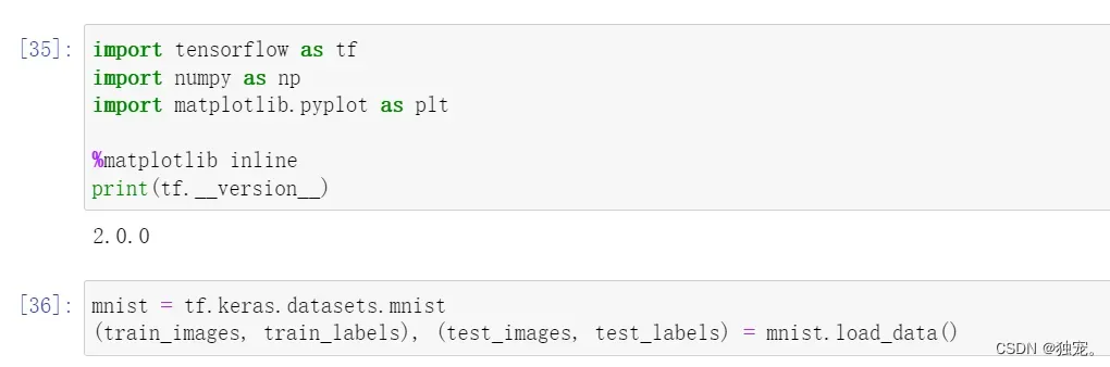
加载数据
import tensorflow as tf
import numpy as np
import matplotlib.pyplot as plt

%matplotlib inline
print(tf.__version__)
mnist = tf.keras.datasets.mnist
(train_images, train_labels), (test_images, test_labels) = mnist.load_data()
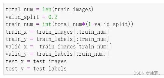
划分数据集
total_num = len(train_images)
valid_split = 0.2
train_num = int(total_num*(1-valid_split))
train_x = train_images[:train_num]
train_y = train_labels[:train_num]
valid_x =  train_images[train_num:]
valid_y = train_labels[train_num:]
test_x = test_images
test_y = test_labels
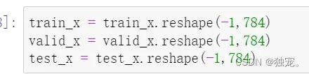
数据整形
train_x = train_x.reshape(-1,784)
valid_x = valid_x.reshape(-1,784)
test_x = test_x.reshape(-1,784)
特征数据归一化
train_x = tf.cast(train_x/255.0,tf.float32)
valid_x = tf.cast(valid_x/255.0,tf.float32)
test_x = tf.cast(test_x/255.0,tf.float32)
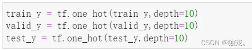
标签数据的one-hot编码
train_y = tf.one_hot(train_y,depth=10)
valid_y = tf.one_hot(valid_y,depth=10)
test_y = tf.one_hot(test_y,depth=10)
建立模型
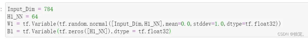
Input_Dim = 784
H1_NN = 64
W1 = tf.Variable(tf.random.normal([Input_Dim,H1_NN],mean=0.0,stddev=1.0,dtype=tf.float32))
B1 = tf.Variable(tf.zeros([H1_NN]),dtype = tf.float32)
创建要优化的变量
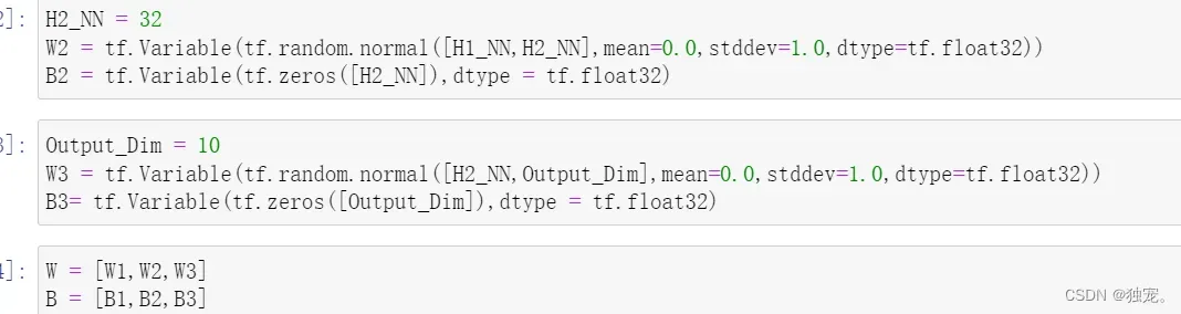
H2_NN = 32
W2 = tf.Variable(tf.random.normal([H1_NN,H2_NN],mean=0.0,stddev=1.0,dtype=tf.float32))
B2 = tf.Variable(tf.zeros([H2_NN]),dtype = tf.float32)
Output_Dim = 10
W3 = tf.Variable(tf.random.normal([H2_NN,Output_Dim],mean=0.0,stddev=1.0,dtype=tf.float32))
B3= tf.Variable(tf.zeros([Output_Dim]),dtype = tf.float32)
W = [W1,W2,W3]
B = [B1,B2,B3]
定义模型前向计算
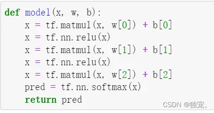
def model(x, w, b):
    x = tf.matmul(x, w[0]) + b[0]
    x = tf.nn.relu(x)
    x = tf.matmul(x, w[1]) + b[1]
    x = tf.nn.relu(x)
    x = tf.matmul(x, w[2]) + b[2]
    pred = tf.nn.softmax(x)
    return pred
定义损失函数
定义交叉熵损失函数
def loss(x, y, w, b):
    pred = model(x, w, b)
    loss_ = tf.keras.losses.categorical_crossentropy(y_true=y, y_pred=pred)
    return tf.reduce_mean(loss_)
设置训练超参数
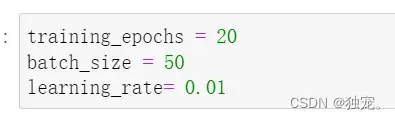
training_epochs = 20
batch_size = 50
learning_rate= 0.01
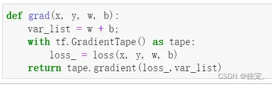
定义梯度计算函数
def grad(x, y, w, b):
    var_list = w + b;
    with tf.GradientTape() as tape:
        loss_ = loss(x, y, w, b)
    return tape.gradient(loss_,var_list)
选择优化器
optimizer = tf.keras.optimizers.Adam(learning_rate=learning_rate)
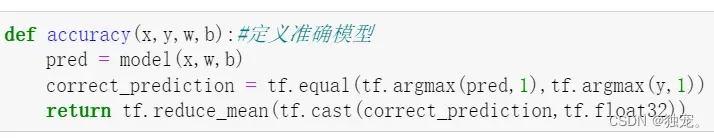
定义精度
def accuracy(x,y,w,b):#定义准确模型
    pred = model(x,w,b)
    correct_prediction = tf.equal(tf.argmax(pred,1),tf.argmax(y,1))
    return tf.reduce_mean(tf.cast(correct_prediction,tf.float32))
训练模型
steps = int(train_num/batch_size)#总次数
loss_list_train = []#定义函数
loss_list_valid = []
acc_list_train = []
acc_list_valid = []
for epoch in range (training_epochs):#循环
for step in range(steps):
xs = train_x[step*batch_size:(step+1)*batch_size]#训练模型的计算
ys = train_y[step*batch_size:(step+1)*batch_size]
grads = grad(xs,ys,W,B)#梯度计算
optimizer.apply_gradients(zip(grads, W+B))
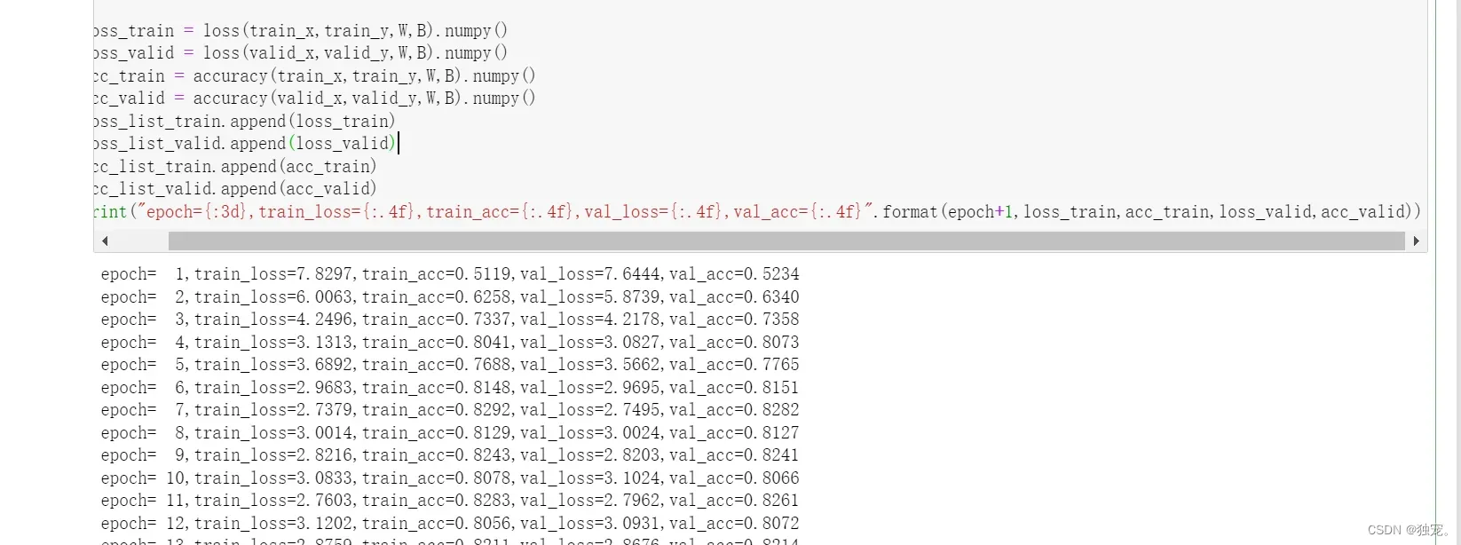
loss_train = loss(train_x,train_y,W,B).numpy()
loss_valid = loss(valid_x,valid_y,W,B).numpy()
acc_train = accuracy(train_x,train_y,W,B).numpy()
acc_valid = accuracy(valid_x,valid_y,W,B).numpy()
loss_list_train.append(loss_train)
loss_list_valid.append(loss_valid)
acc_list_train.append(acc_train)
acc_list_valid.append(acc_valid)
print("epoch={:3d},train_loss={:.4f},train_acc={:.4f},val_loss={:.4f},val_acc={:.4f}".format(epoch+1,loss_train,acc_train,loss_valid,acc_valid))
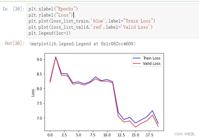
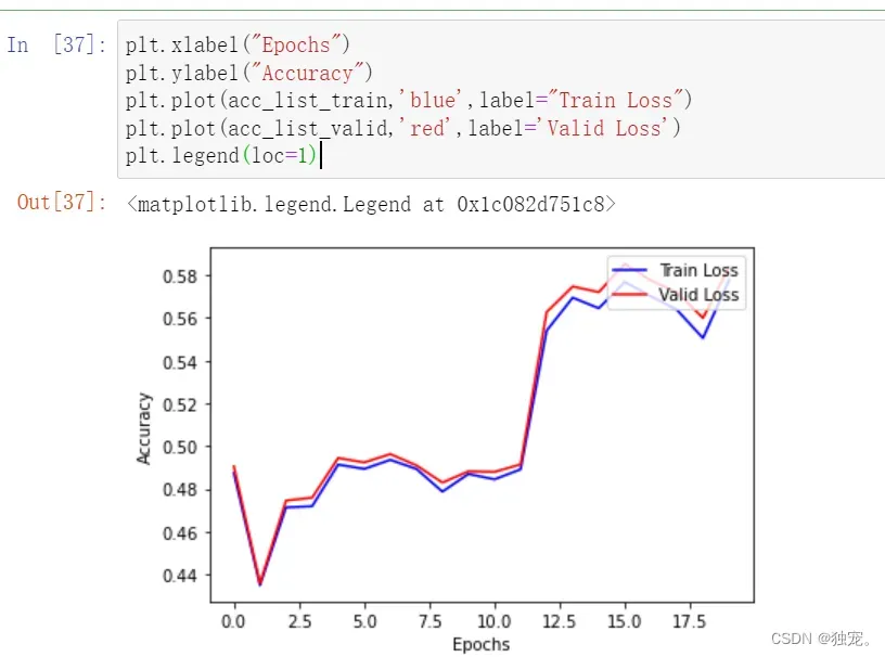
plt.xlabel("Epochs")
plt.ylabel("Loss")
plt.plot(loss_list_train,'blue',label="Train Loss")
plt.plot(loss_list_valid,'red',label='Valid Loss')
plt.legend(loc=1)
plt.xlabel("Epochs")
plt.ylabel("Accuracy")
plt.plot(acc_list_train,'blue',label="Train Loss")
plt.plot(acc_list_valid,'red',label='Valid Loss')
plt.legend(loc=1)
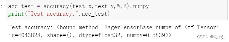
acc_test = accuracy(test_x,test_y,W,B).numpy
print("Test accuracy:",acc_test)
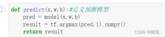
def predict(x,w,b):#定义预测模型
    pred = model(x,w,b)
    result = tf.argmax(pred,1).numpy()
    return result
pred_test=predict(test_x,W,B)

pred_test[0]
import matplotlib.pyplot as plt
import numpy as np
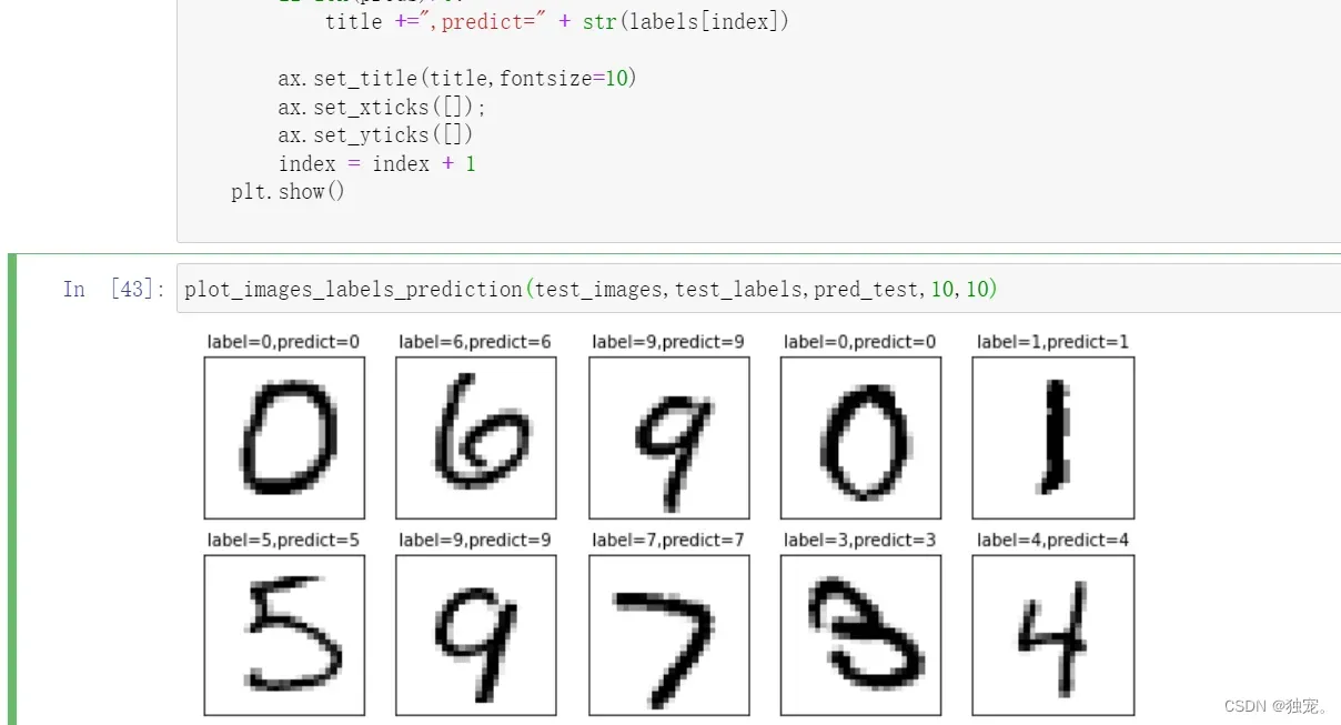
def plot_images_labels_prediction(images,
labels,
preds,
index=0,
num=10):
fig = plt.gcf() #获取当前的图表
fig.set_size_inches(10,4)
if num > 10:
num = 10 #最多显示十个子图
for i in range(0,num):
ax = plt.subplot(2,5,i+1) #获取当前要处理的子图
ax.imshow(np.reshape(images[index],(28,28)),cmap='binary')
title = "label=" + str(labels[index])
if len(preds)>0:
title +=",predict=" + str(labels[index])
ax.set_title(title,fontsize=10)
ax.set_xticks([]);
ax.set_yticks([])
index = index + 1
plt.show()
plot_images_labels_prediction(test_images,test_labels,pred_test,10,10)
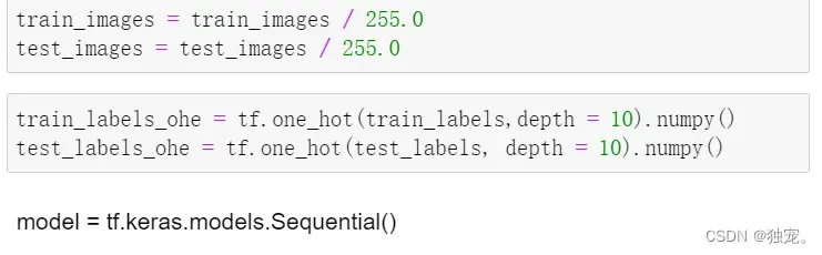
train_images = train_images / 255.0
test_images = test_images / 255.0
train_labels_ohe = tf.one_hot(train_labels,depth = 10).numpy()
test_labels_ohe = tf.one_hot(test_labels, depth = 10).numpy()
创建一个新的序列模型
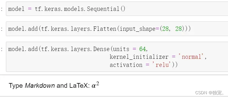
model = tf.keras.models.Sequential()
添加输入层
model.add(tf.keras.layers.Flatten(input_shape=(28, 28)))
添加隐藏层
model.add(tf.keras.layers.Dense(units = 64,
                               kernel_initializer = 'normal',
                               activation = 'relu'))
model.add(tf.keras.layers.Dense(units = 32,
                               kernel_initializer = 'normal',
                               activation = 'relu'))
添加输出层
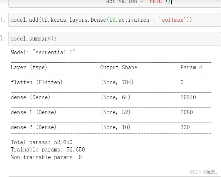
model.add(tf.keras.layers.Dense(10,activation = 'softmax'))
型号汇总
model.summary()
定义训练模式
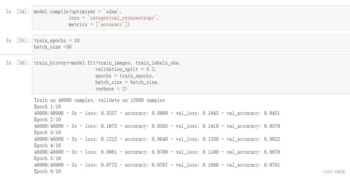
model.compile(optimizer = 'adam',
             loss = 'categorical_crossentropy',
             metrics = ['accuracy'])
设置训练参数
train_epochs = 10
batch_size =30
模型训练
train_history=model.fit(train_images, train_labels_ohe,
                       validation_split = 0.2,
                       epochs = train_epochs,
                       batch_size = batch_size,
                       verbose = 2)
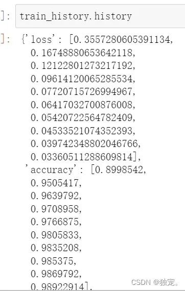
训练过程指标数据
train_history.history
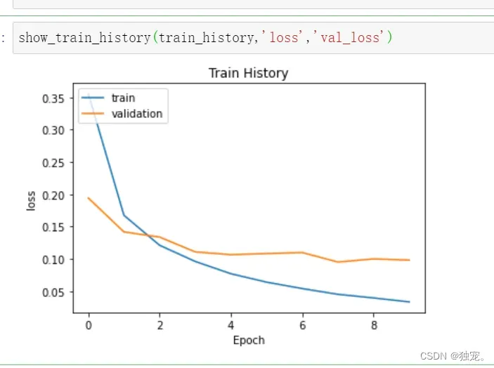
训练过程指标的可视化
import matplotlib.pyplot as plt
def show_train_history(train_history,train_metric,val_metric):
    plt.plot(train_history.history[train_metric])
    plt.plot(train_history.history[val_metric])
    plt.title('Train History')
    plt.ylabel(train_metric)
    plt.xlabel('Epoch')
    plt.legend(['train','validation'],loc='upper left')
    plt.show()
show_train_history(train_history,'loss','val_loss')
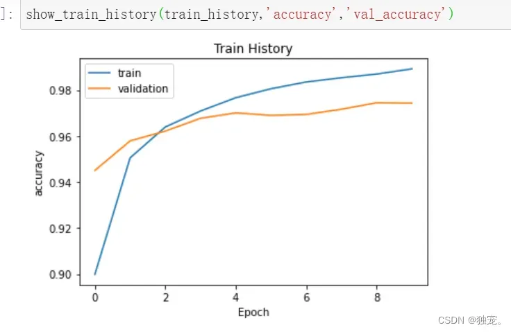
show_train_history(train_history,'accuracy','val_accuracy')
评价模型
test_loss,test_acc = model.evaluate(test_images,test_labels_ohe,verbose = 2)
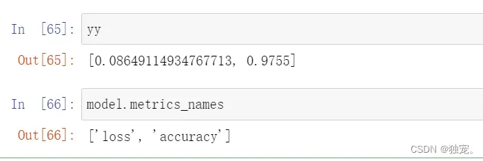
模型的指标
yy=model.evaluate(test_images,test_labels_ohe,verbose=2)
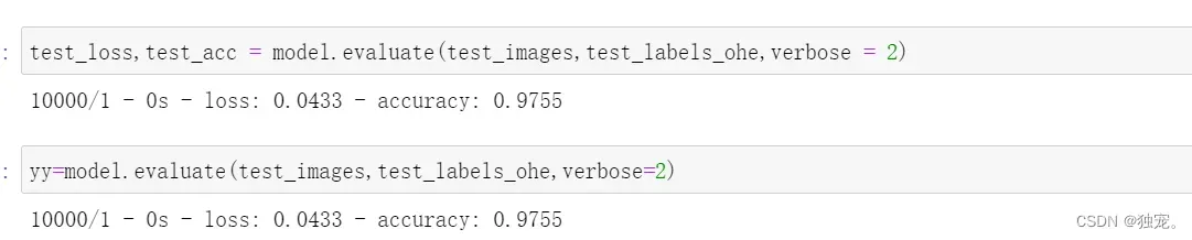
yy
model.metrics_names
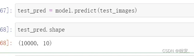
应用模型
test_pred = model.predict(test_images)
test_pred.shape
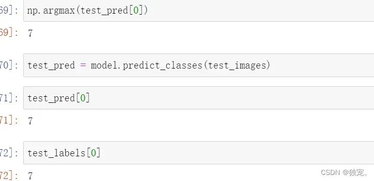
np.argmax(test_pred[0])
应用模型
test_pred = model.predict_classes(test_images)
test_pred[0]
test_labels[0]
文章出处登录后可见!
已经登录?立即刷新