BIC贝叶斯信息准则（用于解决ARIMA模型中q、p参数选择问题）

贝叶斯信息准则，也称为Bayesian Information Criterion(BIC)

1.定义和公式

其中k为模型参数的个数，n为样本的数量，L为似然函数。

模型评估标准：BIC值越低越好。

p和q越大时，参数越多，k越大。所以使k越小，p和q越小，保证模型越好。

L越大，使BIC的值越小，所以似然函数越大越好。

二、代码实现

开发环境：Jupyter Anaconda3

首先需要训练一个ARIMA模型来进行估计，这里我选择使用2015年至2020年道琼斯的时间序列数据集。

1、先导入所需第三方库及依赖

%load_ext autoreload
%autoreload 2
%matplotlib inline
%config InlineBackend.figure_format='retina'
 
from __future__ import absolute_import, division, print_function
import sys
import os
 
import pandas as pd
import numpy as np

 
# TSA from Statsmodels
import statsmodels.api as sm
import statsmodels.formula.api as smf
import statsmodels.tsa.api as smt
 
# Display and Plotting
import matplotlib.pylab as plt
import seaborn as sns
 
pd.set_option('display.float_format', lambda x: '%.5f' % x) # pandas
np.set_printoptions(precision=5, suppress=True) # numpy
 
pd.set_option('display.max_columns', 100)
pd.set_option('display.max_rows', 100)
 
# seaborn plotting style
sns.set(style='ticks', context='poster')

2、导入数据并做一下数据预处理

filename_ts = 'data.csv'
ts_df = pd.read_csv(filename_ts, index_col=0, parse_dates=[0])
n_sample = ts_df.shape[0]
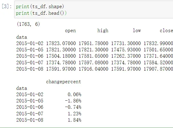
print(ts_df.shape)
print(ts_df.head())

处理后的时间序列数据集如下所示：

3、设置置信区间和需要训练的列

这里我选择闭盘的数据close列

n_train=int(0.95*n_sample)+1
n_forecast=n_sample-n_train
#ts_df
ts_train = ts_df.iloc[:n_train]['close']
ts_test = ts_df.iloc[n_train:]['close']
print(ts_train.shape)
print(ts_test.shape)
print("Training Series:", "\n", ts_train.tail(), "\n")
print("Testing Series:", "\n", ts_test.head())

4、模型评估

获得训练数据集后，您可以执行模型评估

#模型评估
# Fit the model
arima200 = sm.tsa.SARIMAX(ts_train, order=(1,0,0))#order里边的三个参数p,d,q
model_results = arima200.fit()#fit模型

BIC

这里我之前通过绘制ACF和PACF的图像对p、q值的取值范围有了一定的了解，所以p、q值的最大范围做了最小限定。

import itertools
#当多组值都不符合时，遍历多组值，得出最好的值
p_min = 0
d_min = 0
q_min = 0
p_max = 2
d_max = 0
q_max = 10
 
# Initialize a DataFrame to store the results
results_bic = pd.DataFrame(index=['AR{}'.format(i) for i in range(p_min,p_max+1)],
                           columns=['MA{}'.format(i) for i in range(q_min,q_max+1)])
 
for p,d,q in itertools.product(range(p_min,p_max+1),
                               range(d_min,d_max+1),
                               range(q_min,q_max+1)):
    if p==0 and d==0 and q==0:
        results_bic.loc['AR{}'.format(p), 'MA{}'.format(q)] = np.nan
        continue
     
    try:
        model = sm.tsa.SARIMAX(ts_train, order=(p, d, q),
                               #enforce_stationarity=False,
                               #enforce_invertibility=False,
                              )
        results = model.fit()
        results_bic.loc['AR{}'.format(p), 'MA{}'.format(q)] = results.bic
    except:
        continue
results_bic = results_bic[results_bic.columns].astype(float)

可以看一下BIC的输出范围，值越小（黑色区域）越符合，

fig, ax = plt.subplots(figsize=(20, 20))
ax = sns.heatmap(results_bic,
                 mask=results_bic.isnull(),
                 ax=ax,
                 annot=True,
                 fmt='.2f',
                 );
ax.set_title('BIC');

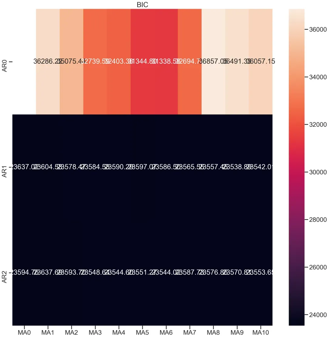
这里可以看出我的BIC值范围，其中纵轴AR为自回归模型输出（q的范围），MA为移动平均模型输出（p的范围）

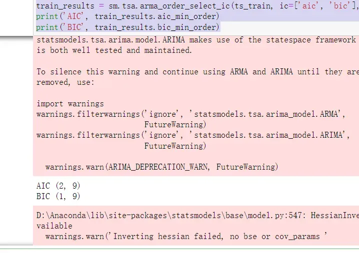
最后输出BIC所判定的p和q的值为1和9。另外还输出了AIC所判定的结果进行对比（在这里不介绍AIC了）。最后我还是通过观察PACF和ACF来进行最终抉择选择BIC输出的q、p值作为参数。

train_results = sm.tsa.arma_order_select_ic(ts_train, ic=['aic', 'bic'], trend='nc', max_ar=2, max_ma=10)
print('AIC', train_results.aic_min_order)
print('BIC', train_results.bic_min_order)

参考https://www.cnblogs.com/tianqizhi/p/9277376.html