注意:本篇为50天后的Java自学笔记扩充,内容不再是基础数据结构内容而是机器学习中的各种经典算法。这部分博客更侧重于笔记以方便自己的理解,自我知识的输出明显减少,若有错误欢迎指正!
目录
一、关于集成学习
1.1 集成学习
所谓集成学习(ensemble learning)给人的感觉就是“ 以多胜优 ”,走群众的路线,众志成城,各自贡献自己的想法并相辅相成。专业来说,进行学习的过程中并不依赖某一个学习器,而是结合多个不同的学习器,或者同个学习器的不同参数环境,一般会获得比任意单个学习器都要好的性能,尤其是在这些学习器都是” 弱学习器 “的时候提升效果会很明显。(所谓弱学习器就是一个学习效率不太好,识别率只能略微超过50%的一类学习器)
西瓜书关于Boosting方面做了一个经典的分析(见公式8.1的推演),即假设有一个二分类问题\(y \in\{-1,+1\}\)和真实函数\(f\),假定这个基本分类器\(h(x_{i})\)的错误率为\(\epsilon\),即\(P(h_{i}(x)≠f(x))=\epsilon\)。然后我们利用简单投票的法则,结合\(T\)个基分类器,若有超过一半以上的基分离器正确,那么集成就是成功的:\[H(x)=\operatorname{sign}\left(\sum_{i=1}^{M} h_{i}(x)\right)\] (上式使用求和对于仅仅为+1/-1的二分类取值可以实现投票效果)
继续假设基学习器之间的错误率是相互独立的,那么可有Hoeffding不等式可得集成的错误率为:\[P(H(x) \neq f(x)) \leq \exp \left(-\frac{1}{2} M(1-2 \epsilon)^{2}\right)\] 关于Hoeffding不等式,鄙人数学能力有限暂且不给出说明,这里上面给出西瓜书的说明只是为了引出下面结论:上式表现出来随着个体学习器数目\(T\)的增大,集成错误率是呈现指数级的下降,最终趋于0。
当然上面的介绍是在每个学习器的误差相互独立的条件下推演出来的,但是在现实中,我们采用集成学习设计的诸多学习器都是针对同一个问题学习得到的,因此其彼此之间不可能完全独立。因此我们总是尽可能使得其变得独立,或者说增加基学习器的“多样性”。这些是目前集成学习正在突破的方向。而今天我们学习的Boosting正是针对个体学习器之间存在强依赖关系、必须串行生成的序列化方法。(与之对立的还有弱依赖、同时生成的并行化方法的Bagging和Random Forest)
1.2 AdaBoost的过程
Boosting作为将弱学习器叠加为强学习机的算法,是通过将先前的基学习器的错误样本在后续训练中持续收到关注的方法来调整和训练下一个样本集。其中,AdaBoost(Adapted Boost)是Boosting族算法的一个代表,其采用了指数作为衡量权重的代表,后续在代码中我会给出这个衡量公式。
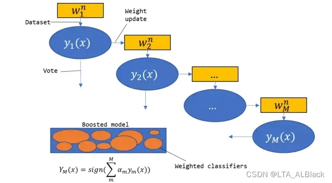
AdaBoost的过程可通过下图表示,首先我们拥有一个基本的数据集\(w_{1}^{n}\),最初的时候有个默认的分类权值体系,表述着当前数据的信息。之后通过一次非常简单的、快速的学习过程得到一个弱学习分类器\(y_{1}(x)\)。因为\(y_{1}(x)\)的准确率比较低,因此我们发现了一些失败的测试数据,于是改变失败的数据权值。后续的数据集\(w_{2}^{n}\)继承\(w_{1}^{n}\)的数据,只不过在后续学习得到学习分类器\(y_{2}(x)\)的过程中是基于改变后的数据权值体系。
综上,通过数据集的\(M\)个版本,我们训练出了\(M\)个基分类器。而在最终得到全局的集成模型(或者说最终的学习分类器)的时候,\(M\)个学习分类器都将起作用,即每个分类器的加权(分类指标)和。全过程宛如串行与并行的组合:
- 学习分类器每次基于以往数据的正确性对数据进行权值更新,从而迭代为新的分类器(串行)
- 最终获得最后分类器的时候,每个分类器会并行进行加权投票(并行)
1.3 代码总览目录
由于今天的代码量非常庞大,定义了若干的类,所以在开始展示代码与逻辑之前通过一个草图先预览下我们接下来要做的事情:
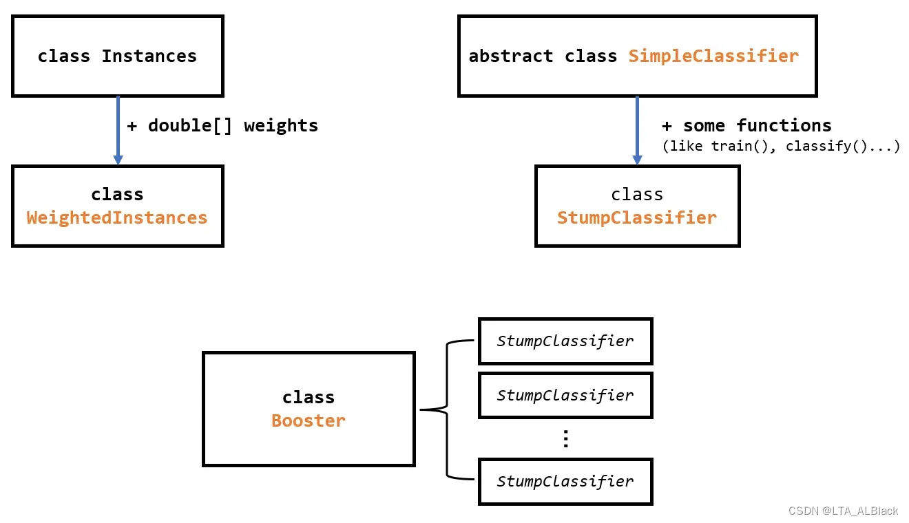
因为AdaBoost是引入了权值的数据集,为了方便后续代码的编写,我们对于常规的Instance数据集进行了继承构造出了WeightedInstance类,这部分将在第二部分讲述。同时第二部分我会通过权值数组来简单说说我对于权值调整的理解与实现。
为了能够象征表示每个分类器共有属性,创建了抽象类SimpleClassifier,并定义了一些分类器的通用操作:比如算准确性、算错误总权…这个在第三部分描述
AdaBoost的集成器是由若干树桩树桩构成的,于是继承了一般分类器SimpleClassifier的特性,进一步实际定义了树桩分类器类StumpClassifier,包括了树桩分类器的二元分割方法。这个在文章第四部分。
最后设计了集成器Booster类,将若干StumpClassifier构造的树桩对象通过串行集成到了一体,并且实现了并行的测试数据分类。这个在文章第五部分。
二、基础代码准备-带权数据集
2.1 基础准备
之前学习的过程中我们都是使用Instances这个数据作为数据集的类,但是在adaboosting过程中因为数据集的每一行都应当具有其权值,而这个权值属于算法定义而非数据本身携带,因此为了方便,这里继承了Instances类并将其扩充为支持 额外附加一项权值属性 的数据集。
public class WeightedInstances extends Instances{

	/**
	 * Weights.
	 */
	private double[] weights;

	/**
	 ******************
	 * Getter.
	 *
	 * @param paraIndex
	 *            The given index.
	 * @return The weight of the given index.
	 ******************
	 */
	public double getWeight(int paraIndex) {
		return weights[paraIndex];
	} // Of getWeight


	//...other function...


} // Of class WeightedInstances
只需要在一般的Instance关系表旁附带一个权值数组即可。
一些基础的构造:
    /**
	 ******************
	 * The first constructor.
	 *
	 * @param paraFileReader
	 *            The given reader to read data from file.
	 ******************
	 */
	public WeightedInstances(FileReader paraFileReader) throws Exception {
		super(paraFileReader);
		setClassIndex(numAttributes() - 1);

		// Initialize weights
		weights = new double[numInstances()];
		double tempAverage = 1.0 / numInstances();
		for (int i = 0; i < weights.length; i++) {
			weights[i] = tempAverage;
		} // Of for i
		System.out.println("Instances weights are: " + Arrays.toString(weights));
	} // Of the first constructor

	/**
	 ******************
	 * The second constructor.
	 *
	 * @param paraInstances
	 *            The given instance.
	 ******************
	 */
	public WeightedInstances(Instances paraInstances) {
		super(paraInstances);
		setClassIndex(numAttributes() - 1);

		// Initialize weights
		weights = new double[numInstances()];
		double tempAverage = 1.0 / numInstances();
		for (int i = 0; i < weights.length; i++) {
			weights[i] = tempAverage;
		} // Of for i
		System.out.println("Instances weights are: " + Arrays.toString(weights));
	} // Of the second constructor
实现了基于文件指针与Instance类型的两个构造器,后者用于同类拷贝。注意这里要super调用父级的构造函数,将参数传给Instance类,我们没必要关心这个参数是怎么读入到Instance类中的细节,我们只需要关系我们的之类相比父级多出的构造操作就好了。
其实多出来的内容不算多,确定决策列(标签所在的属性列);给关系表的附加数组weights赋值。我们这里定义的每个数据项的权值为\(\frac{1}{n}\),即所有权值和要保持1.0。
2.2 权值调整规则
	/**
	 ******************
	 * Adjust the weights.
	 *
	 * @param paraCorrectArray
	 *            Indicate which instances have been correctly classified.
	 * @param paraAlpha
	 *            The weight of the last classifier.
	 ******************
	 */
	public void adjustWeights(boolean[] paraCorrectArray, double paraAlpha) {
		// Step 1. Calculate alpha.
		double tempIncrease = Math.exp(paraAlpha);

		// Step 2. Adjust.
		double tempWeightsSum = 0; // For normalization.
		for (int i = 0; i < weights.length; i++) {
			if (paraCorrectArray[i]) {
				weights[i] /= tempIncrease;
			} else {
				weights[i] *= tempIncrease;
			} // Of if
			tempWeightsSum += weights[i];
		} // Of for i

		// Step 3. Normalize.
		for (int i = 0; i < weights.length; i++) {
			weights[i] /= tempWeightsSum;
		} // Of for i

		System.out.println("After adjusting, instances weights are: " + Arrays.toString(weights));
	} // Of adjustWeights
这个代码是基于paraCorrectArray数组对权值进行调整的代码,参考参数paraAlpha。
这个过程可每一行的权值决断可以简化为下面这样的函数\(f(x_{i})\):\[f(x_{i})=\left\{\begin{array}{cc}
w_{i} e^{-\alpha}, & x_{i} \text { is correct } \\
w_{i} e^{\alpha}, & x_{i} \text { is wrong }
\end{array}\right. \tag{1} \] 上式中\(x_i\)象征着第\(i\)行数据,而\(w_{i}\)表示第\(i\)行数据的权值,而\(f(x_{i})\)表示在影响因子\(\alpha\)(关于这个值在集成器部分会具体介绍)影响下,权值\(w_{i}\)的增益或者衰减结果。在程序中,\(x_i\)的分类成功与否是通过一个布尔数组来表示的。
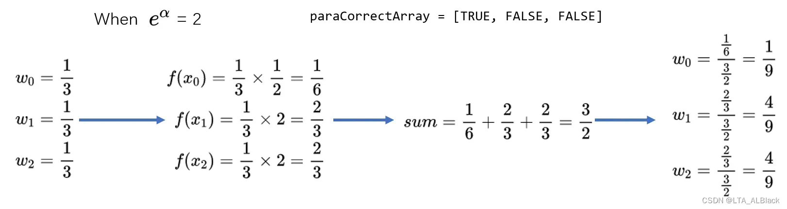
最终调整后,单条数据的权值并不是\(f(x_{i})\),因为这样没法保证总权为1.0,因此数组的任意第\(i\)行的权值应该为\(\frac{f(x_{i})}{\sum_{i=1}^{n} f\left(x_{i}\right)}\),从而确保总权值保持不变。
通过这个公式可基本进行分析,当\(\alpha > 0\),通过指数函数的基本特性可知,分类器判断正确的数据行的基础权会相比之前\(w_{i}\)有所下降,而失败的数据基础权\(w_{i}\)会有所提升。如此一来,之前每个行相同的权值关系就会被破坏,如果这时把所有行的新权值\(f(x_{i})\)求和并以和作为底,那么势必在保持总权为1.0的情况下,基分类器判断正确数据行的权值会下降,失败的数据行权值会上升。(下图是一个例子)
2.3 输出测试
这部分没什么特别的含义,只是测试一下此类的输出情况,同时测试某种\(\alpha\)影响下的权值调整(对于最终的AdaBoosting代码无影响):
    /**
	 ******************
	 * For display.
	 ******************
	 */
	public String toString() {
		String resultString = "I am a weighted Instances object.\r\n" + "I have " + numInstances() + " instances and "
				+ (numAttributes() - 1) + " conditional attributes.\r\n" + "My weights are: " + Arrays.toString(weights)
				+ "\r\n" + "My data are: \r\n" + super.toString();

		return resultString;
	} // Of toString

	/**
	 ******************
	 * For unit test.
	 *
	 * @param args
	 *            Not provided.
	 ******************
	 */
	public static void main(String args[]) {
		WeightedInstances tempWeightedInstances = null;
		String tempFilename = "d:/Java DataSet/iris.arff";
		try {
			FileReader tempFileReader = new FileReader(tempFilename);
			tempWeightedInstances = new WeightedInstances(tempFileReader);
			tempFileReader.close();
		} catch (Exception exception1) {
			System.out.println("Cannot read the file: " + tempFilename + "\r\n" + exception1);
			System.exit(0);
		} // Of try

		System.out.println(tempWeightedInstances.toString());

		tempWeightedInstances.adjustWeightsTest();
	} // Of main
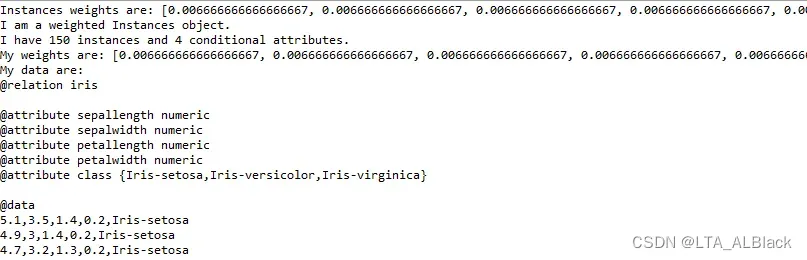
基本输出(后续数据不再给出,这里的0.00667正是\(\frac{1}{150}\)的结果):
权调整测试案例中,我们假设正确\失败情况各半,并且\(\alpha = 0.3\)。
	/**
	 ******************
	 * Test the method.
	 ******************
	 */
	public void adjustWeightsTest() {
		boolean[] tempCorrectArray = new boolean[numInstances()];
		for (int i = 0; i < tempCorrectArray.length / 2; i++) {
			tempCorrectArray[i] = true;
		} // Of for i

		double tempWeightedError = 0.3;

		adjustWeights(tempCorrectArray, tempWeightedError);

		System.out.println("After adjusting");

		System.out.println(toString());
	} // Of adjustWeightsTest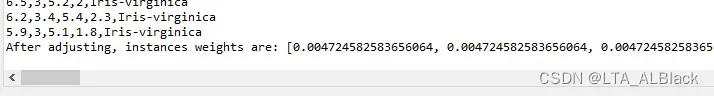
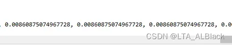
正确数据的权值变为0.00472,而错误数据的权值变为0.00861,符合上述分析的\(\alpha > 0\)时的正确数据与错误数据的权变化情况。
三、基分类器的抽象类
3.1 基本参数说明与抽象方法定义
本类作为抽象类,主要目的是为后续的分类器构造提供一些可用的部件,从而提高分类器创建之可重用性。
public abstract class SimpleClassifier {

	/**
	 * The index of the current attribute.
	 */
	int selectedAttribute;

	/**
	 * Weighted data.
	 */
	WeightedInstances weightedInstances;

	/**
	 * The accuracy on the training set.
	 */
	double trainingAccuracy;

	/**
	 * The number of classes. For binary classification it is 2.
	 */
	int numClasses;

	/**
	 * The number of instances.
	 */
	int numInstances;

	/**
	 * The number of conditional attributes.
	 */
	int numConditions;

	/**
	 * For random number generation.
	 */
	Random random = new Random();

	/**
	 ******************
	 * The first constructor.
	 *
	 * @param paraWeightedInstances
	 *            The given instances.
	 ******************
	 */
	public SimpleClassifier(WeightedInstances paraWeightedInstances) {
		weightedInstances = paraWeightedInstances;

		numConditions = weightedInstances.numAttributes() - 1;
		numInstances = weightedInstances.numInstances();
		numClasses = weightedInstances.classAttribute().numValues();
	}// Of the first constructor

    // other function...

} // Of class SimpleClassifier
- selectedAttribute选用的划分属性(参考昨日的决策树的分叉思想)
- weightedInstances带权数据集
- trainingAccuracy当前分类器本身的训练准确性
- numClasses\numInstances\numConditions数据集属性“三件套”,即标签数目(决策属性列可用类别的数目)、数据集长度、条件属性个数
作为抽象类就要有抽象类的样子,自然,我们这里也为后续任何分类器共有的训练与分类特征设置了相应的接口:
    /**
	 ******************
	 * Train the classifier.
	 ******************
	 */
	public abstract void train();

	/**
	 ******************
	 * Classify an instance.
	 *
	 * @param paraInstance
	 *            The given instance.
	 * @return Predicted label.
	 ******************
	 */
	public abstract int classify(Instance paraInstance);
train()是分类器的基础构建方法,是构建分类器的触发方法,而外来的数据行要经过这个分类器进行测试时,就需要通过classify接口,获得基于此分类器得到的标签裁决。这些东西都是基于不同分类器会分化的特征,因此在抽象类中只需要定义接口即可。
3.2 通用的准确度计算
准确度的计算无非就将某个测试集的数据到分类得到的模型中去逐个测试,并且看是否和测试集本身(掩住)已知的标签一致。既然我们能这样泛泛描述,那么这个方法应该是所有分类器在测试时共有的特征,因此可以作为实体方法写出来。
注意,Adaboosting构造的基分类器是弱分类器,不同于ID3决策树的模型,弱分类器哪怕是用训练出自己模型的数据集再度作为测试集,最终的结果也不一定是1.0。所以下面测试准确度我们都是用自己训练自己并且自己测试自己。
	/**
	 ******************
	 * Which instances in the training set are correctly classified.
	 *
	 * @return The correctness array.
	 ******************
	 */
	public boolean[] computeCorrectnessArray() {
		boolean[] resultCorrectnessArray = new boolean[weightedInstances.numInstances()];
		for (int i = 0; i < resultCorrectnessArray.length; i++) {
			Instance tempInstance = weightedInstances.instance(i);
			if ((int) (tempInstance.classValue()) == classify(tempInstance)) {
				resultCorrectnessArray[i] = true;
			} // Of if
		} // Of for i
		return resultCorrectnessArray;
	}// Of computeCorrectnessArray
注意,这个地方classify是未定的一个函数引用,这个引用的地址是未定的。随着后续实体类继承了此抽象类并实体定义classify方法,这个classify才会获得一个可调用的函数入口。即实现了函数入口的后绑定——这就是Java的多态。
其通过逐一的遍历,得到了每行训练集数据的分类是否正确的状况数组,返回之。这个数组正是我们刚刚提到的进行权调整的数组。
	/**
	 ******************
	 * Compute the accuracy on the training set.
	 *
	 * @return The training accuracy.
	 ******************
	 */
	public double computeTrainingAccuracy() {
		double tempCorrect = 0;
		boolean[] tempCorrectnessArray = computeCorrectnessArray();
		for (int i = 0; i < tempCorrectnessArray.length; i++) {
			if (tempCorrectnessArray[i]) {
				tempCorrect++;
			} // Of if
		} // Of for i

		double resultAccuracy = tempCorrect / tempCorrectnessArray.length;

		return resultAccuracy;
	}// Of computeTrainingAccuracy
通过computeCorrectnessArray()方法更新了tempCorrectnessArray[ ],于是进行统计,计算整个分类器的准确度。
	 ******************
	 * Compute the weighted error on the training set. It is at least 1e-6 to
	 * avoid NaN.
	 *
	 * @return The weighted error.
	 ******************
	 */
	public double computeWeightedError() {
		double resultError = 0;
		boolean[] tempCorrectnessArray = computeCorrectnessArray();
		for (int i = 0; i < tempCorrectnessArray.length; i++) {
			if (!tempCorrectnessArray[i]) {
				resultError += weightedInstances.getWeight(i);
			} // Of if
		} // Of for i

		if (resultError < 1e-6) {
			resultError = 1e-6;
		} // Of if

		return resultError;
	}// Of computeWeightedError
统计所有的分类出错的数据行的权总和,注意,为了避免极小值导致越界的错误,对于一切过小的值错误或者过小的情况都设置为最底线的1e-6(避免越界的常见技巧)。
这里统计全部的失败权即是下回合调整下一个迭代分类器的\(\alpha\)构造所需的一个材料,这里先卖个关子,因为这个值是一个枢纽,所以我会在后面集成器的时候具体说说其实现含义与步骤。
四、树桩分类器
4.1 树桩分类器的二分分割思想
· 为什么是树桩?
之所以这类分类器我们会称之为“ 树桩 ”,因为这种分类器是没有分支的。AdaBoost当中,树桩分类器只一个二分类器,即只能识别两个标签,而且分类之后没有递归,就简单分出两个孩子而已。显然这样的分类器自身是无法胜任多标签的任务,我们需要通过多个AdaBoost的多个分类器的串行组合来从两个标签扩充到多标签。
树桩分类类似于ID3决策树但是又有不同,相同地方在于:
- 他们都会选定一个条件属性作为自己分类的依据
- 都是通过分析条件属性的可取值来分割数据集
不同地方在于:
- ID3决策树选择这样的条件属性是依靠信息增益原则,而树桩选取分类的参考属性是利用随机数(选谁都行!完全随机,虽然有时参考样例不准确,但是我快啊!我可以反复迭代继承来提高准确率!)
- 树桩分类器仅仅对于所选择的条件属性下属的全部数据进行二分叉(连续数据),比较简单;而ID3决策树会对于所选择的条件属性下属的每个类别进行分叉(比如针对条件属性如果是outlook,我可能会分别分叉sunny、overcast、rainy三个孩子,若是连续数据也会采用某些策略分割,不一定是二分叉)
- ID3决策树在分割后,若孩子不纯且孩子中的数据行数还足够,则会继续分(不断分治);但是树桩只会分一次(要么为什么叫做树桩,对吧),不会递归
· 随机选定属性列
具体来总结这个过程有下图:
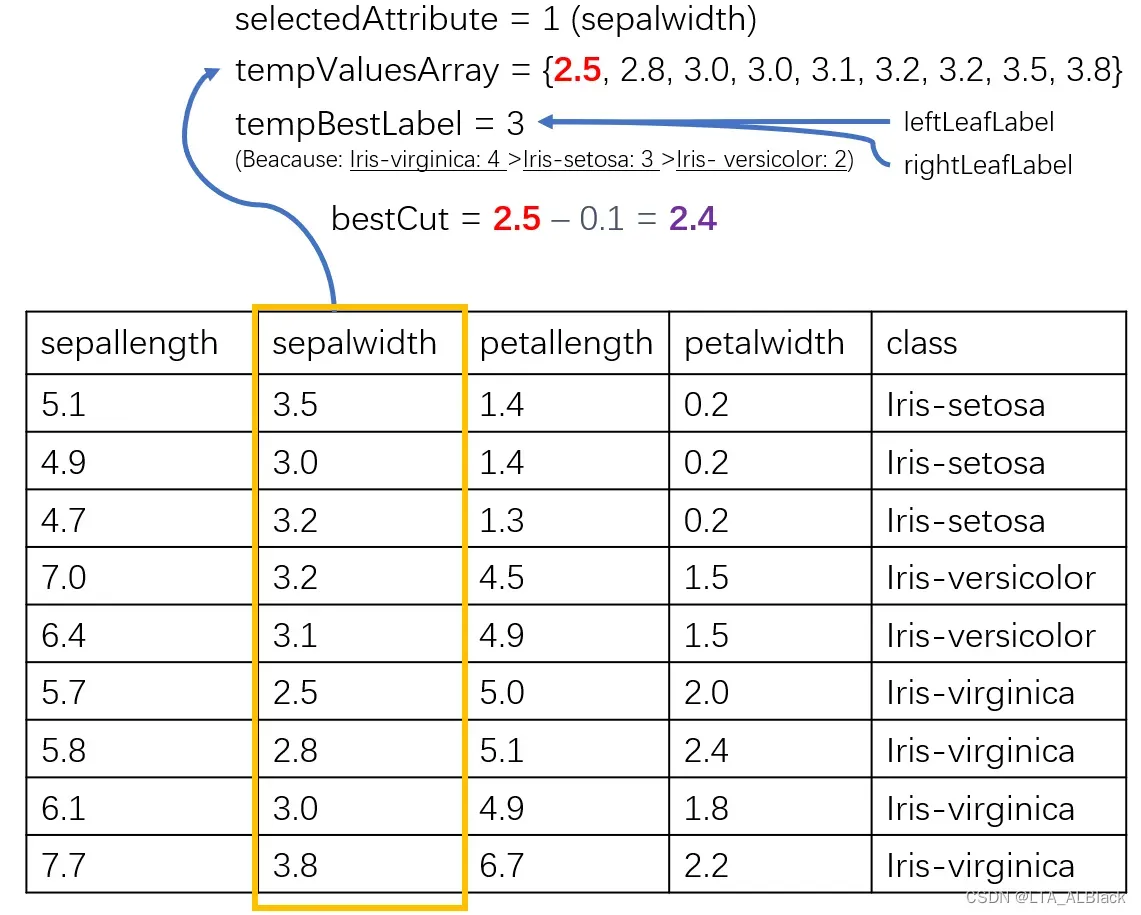
首先随机选择一个属性列,上图中我们选择了第1号列-sepalwidth,然后将此列数据排序得到tempValueArray,之后我们的分割都将基于这个属性列的数据进行考虑。此外我们还需要准备几个关键的变量:
- tempBestLabel 临时的最佳标签。这个变量是通过一次统计操作取得的当前数据集的全部9个数据中权值最大的标签,至于这个统计操作是如何进行的,先卖个关子,在后面具体阐述。
- leftLeafLabel & rightLeafLabel 左\右叶子的最佳标签。记录左右孩子权值最大的标签,初始还未统计,因此初始值为tempBestLabel
- bestCut 最佳切断值。这个变量是用于存放我们切断数组的最佳值,这个值不能与数组中的任何一个元素重叠,从而保证数组能基于这个值不重叠地将数组分为两个不重叠的子集。初始还没有探寻,于是取任何一个不于数组中重叠的值即可。(这里取的首元素-0.1的值,显然不重叠)
· 什么是一次统计操作
这个操作的目的在于选择操作范围的数据集中最佳的标签。首先确定这个范围的数据集有哪些标签,然后对这些标签进行投票。遍历每个数据行,若这个数据行隶属B标签,同时其权值为\(w_{i}\),那么B标签权值就+ \(w_{i}\),最终投票下来权值最高的标签就是我们认定的最佳标签。
从这种分析不难看出,一旦一个数据集中某些标签为代表的数据行当初被误判得越多,那么之后分类的时候就更能认为这个标签是一个最标签。而后续我们会了解到,“最佳标签” 是更可能代表一个数据集的。
· 分割
选定的条件属性列中的排序数组(下面都称之为目标数组)中并不是每个位置都是可分的
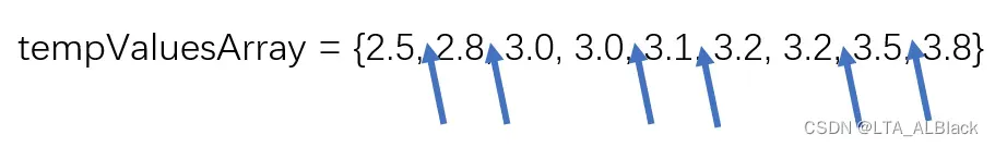
只有存在一个\(x_{i}\)与\(x_{i+1}\),满足\(0≤i<n-1\),并且\(x_{i} ≠x_{i+1}\) 时,这时两数之间才可分,有\(tempCut = \frac{x_{i} + x_{i+1}}{2}\)。这里之所以限制\(x_{i} ≠x_{i+1}\)是因为当\(x_{i} =x_{i+1}\)时有\(tempCut = \frac{x_{i} + x_{i+1}}{2} = x_{i} = x_{i+1}\),这时分割点与数组重合了,违背了最初的假设,无法有效进行分割。
那么我们要选择哪个点进行分割呢?都试下咯
我们定义,在某个分割点的情况下将目标数组分为左右两个部分,而这两个部分中每个单独的数值,在原数据集中都可以唯一地表征某个数据行。言下之意,这个小小的分割点,就可以将我们原本的数据集一分为二。那么好勒,只要分别对于左右两个数据集进行一次统计操作,取得左右数据集的最佳的标签与最佳标签的投票总权。然后把左右的数据集的总权加起来即当前分割的权重,最终我们选择权重最高的那次分割就好了。
用一个图来说明:
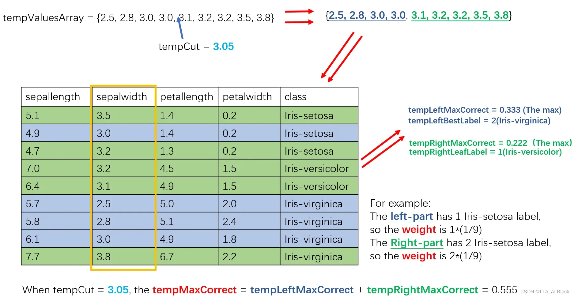
图右侧的tempLeftMaxCorrent = 0.333 是对于 2号标签(也就是Iris-virginia)投票得到的权重,因为这个权值是蓝色(分割的左侧)数据集中最大的,所以我们就选择它作为我们蓝色数据集中的最高权重与最佳标签。
由此,确定tempCut = 3.05的分割之后,我们得到左侧数据集的权为0.333,右侧的为0.222。从而当前的分割权重为0.555。
这就是一次循环的取值,不断循环直到某时分割权重取到最大值,这时分别将最佳左侧数据权存放到leftLeafLabel 最佳右侧权存放到rightLeafLabel 。并将此刻的tempCut存到bestCut
4.2 二分分割代码
这里的属性与我们在讲述思想时用的是同样的名称:
	/**
	 * The best cut for the current attribute on weightedInstances.
	 */
	double bestCut;

	/**
	 * The class label for attribute value less than bestCut.
	 */
	int leftLeafLabel;

	/**
	 * The class label for attribute value no less than bestCut.
	 */
	int rightLeafLabel;

	/**
	 ******************
	 * The only constructor.
	 *
	 * @param paraWeightedInstances
	 *            The given instances.
	 ******************
	 */
	public StumpClassifier(WeightedInstances paraWeightedInstances) {
		super(paraWeightedInstances);
	}// Of the only constructor
只要思想懂,再长代码也水到渠成(这时AdaBoost的代码最难点):
	/**
	 ******************
	 * Train the classifier.
	 ******************
	 */
	public void train() {
		// Step 1. Randomly choose an attribute.
		selectedAttribute = random.nextInt(numConditions);

		// Step 2. Find all attribute values and sort.
		double[] tempValuesArray = new double[numInstances];
		for (int i = 0; i < tempValuesArray.length; i++) {
			tempValuesArray[i] = weightedInstances.instance(i).value(selectedAttribute);
		} // Of for i
		Arrays.sort(tempValuesArray);

		// Step 3. Initialize, classify all instances as the same with the
		// original cut.
		int tempNumLabels = numClasses;
		double[] tempLabelCountArray = new double[tempNumLabels];
		int tempCurrentLabel;

		// Step 3.1 Scan all labels to obtain their counts.
		for (int i = 0; i < numInstances; i++) {
			// The label of the ith instance
			tempCurrentLabel = (int) weightedInstances.instance(i).classValue();
			tempLabelCountArray[tempCurrentLabel] += weightedInstances.getWeight(i);
		} // Of for i

		// Step 3.2 Find the label with the maximal count.
		double tempMaxCorrect = 0;
		int tempBestLabel = -1;
		for (int i = 0; i < tempLabelCountArray.length; i++) {
			if (tempMaxCorrect < tempLabelCountArray[i]) {
				tempMaxCorrect = tempLabelCountArray[i];
				tempBestLabel = i;
			} // Of if
		} // Of for i

		// Step 3.3 The cut is a little bit smaller than the minimal value.
		bestCut = tempValuesArray[0] - 0.1;
		leftLeafLabel = tempBestLabel;
		rightLeafLabel = tempBestLabel;

		// Step 4. Check candidate cuts one by one.
		// Step 4.1 To handle multi-class data, left and right.
		double tempCut;
		double[][] tempLabelCountMatrix = new double[2][tempNumLabels];

		for (int i = 0; i < tempValuesArray.length - 1; i++) {
			// Step 4.1 Some attribute values are identical, ignore them.
			if (tempValuesArray[i] == tempValuesArray[i + 1]) {
				continue;
			} // Of if
			tempCut = (tempValuesArray[i] + tempValuesArray[i + 1]) / 2;

			// Step 4.2 Scan all labels to obtain their counts wrt. the cut.
			// Initialize again since it is used many times.
			for (int j = 0; j < 2; j++) {
				for (int k = 0; k < tempNumLabels; k++) {
					tempLabelCountMatrix[j][k] = 0;
				} // Of for k
			} // Of for j

			for (int j = 0; j < numInstances; j++) {
				// The label of the jth instance
				tempCurrentLabel = (int) weightedInstances.instance(j).classValue();
				if (weightedInstances.instance(j).value(selectedAttribute) < tempCut) {
					tempLabelCountMatrix[0][tempCurrentLabel] += weightedInstances.getWeight(j);
				} else {
					tempLabelCountMatrix[1][tempCurrentLabel] += weightedInstances.getWeight(j);
				} // Of if
			} // Of for i

			// Step 4.3 Left leaf.
			double tempLeftMaxCorrect = 0;
			int tempLeftBestLabel = 0;
			for (int j = 0; j < tempLabelCountMatrix[0].length; j++) {
				if (tempLeftMaxCorrect < tempLabelCountMatrix[0][j]) {
					tempLeftMaxCorrect = tempLabelCountMatrix[0][j];
					tempLeftBestLabel = j;
				} // Of if
			} // Of for i

			// Step 4.4 Right leaf.
			double tempRightMaxCorrect = 0;
			int tempRightBestLabel = 0;
			for (int j = 0; j < tempLabelCountMatrix[1].length; j++) {
				if (tempRightMaxCorrect < tempLabelCountMatrix[1][j]) {
					tempRightMaxCorrect = tempLabelCountMatrix[1][j];
					tempRightBestLabel = j;
				} // Of if
			} // Of for i

			// Step 4.5 Compare with the current best.
			if (tempMaxCorrect < tempLeftMaxCorrect + tempRightMaxCorrect) {
				tempMaxCorrect = tempLeftMaxCorrect + tempRightMaxCorrect;
				bestCut = tempCut;
				leftLeafLabel = tempLeftBestLabel;
				rightLeafLabel = tempRightBestLabel;
			} // Of if
		} // Of for i

		System.out.println("Attribute = " + selectedAttribute + ", cut = " + bestCut + ", leftLeafLabel = "
				+ leftLeafLabel + ", rightLeafLabel = " + rightLeafLabel);
	}// Of train
4.3 测试数据分类以及基本测试
	/**
	 ******************
	 * Classify an instance.
	 *
	 * @param paraInstance
	 *            The given instance.
	 * @return Predicted label.
	 ******************
	 */
	public int classify(Instance paraInstance) {
		int resultLabel = -1;
		if (paraInstance.value(selectedAttribute) < bestCut) {
			resultLabel = leftLeafLabel;
		} else {
			resultLabel = rightLeafLabel;
		} // Of if
		return resultLabel;
	}// Of classify
树桩分类器因为仅仅实现数据一次的二分,因此对于单行数据的分类就非常非常简单,只需要判断导入的数据行的selectedAttribute列数据大小,判断其所属区间从而判断其标签。
因为准确度测试的代码已经在抽象的超类中说明了,故这里不必再描述。下面试着测试下数据效果:
    /**
	 ******************
	 * For display.
	 ******************
	 */
	public String toString() {
		String resultString = "I am a stump classifier.\r\n" + "I choose attribute #" + selectedAttribute
				+ " with cut value " + bestCut + ".\r\n" + "The left and right leaf labels are " + leftLeafLabel
				+ " and " + rightLeafLabel + ", respectively.\r\n" + "My weighted error is: " + computeWeightedError()
				+ ".\r\n" + "My weighted accuracy is : " + computeTrainingAccuracy() + ".";

		return resultString;
	}// Of toString

	/**
	 ******************
	 * For unit test.
	 *
	 * @param args
	 *            Not provided.
	 ******************
	 */
	public static void main(String args[]) {
		WeightedInstances tempWeightedInstances = null;
		String tempFilename = "D:/Java DataSet/iris.arff";
		try {
			FileReader tempFileReader = new FileReader(tempFilename);
			tempWeightedInstances = new WeightedInstances(tempFileReader);
			tempFileReader.close();
		} catch (Exception ee) {
			System.out.println("Cannot read the file: " + tempFilename + "\r\n" + ee);
			System.exit(0);
		} // Of try

		StumpClassifier tempClassifier = new StumpClassifier(tempWeightedInstances);
		tempClassifier.train();
		System.out.println(tempClassifier);

		System.out.println(Arrays.toString(tempClassifier.computeCorrectnessArray()));
	}// Of main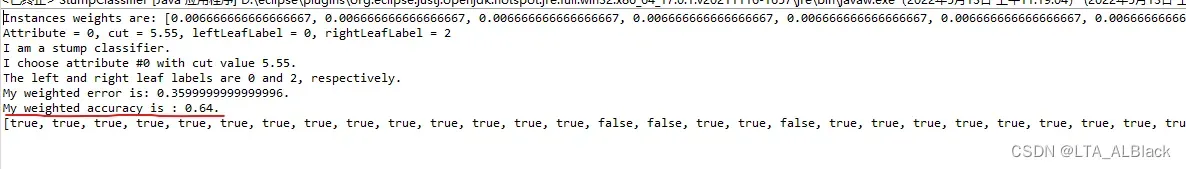
这是某次分类的结果,选择了第0列sepallength属性进行分割,分割的中间值是5.5,分割的左右数据集最佳的标签分别是0号标签Iris-setosa与2号标签Iris-virginica;最终正确率为0.64。
虽然每次选择用于分割的条件属性列是不同的,但是每列的数据是确定的,因此bestCut也是一定的,所以基分类器分类的数据集如果有\(M\)列的话,或者说有\(M\)个条件属性的话,那么最终也会有\(M\)个可能的bestCut,对应\(M\)种准确率。通过随机的枚举,我们测试出了下面这张映射表:
| selectedAttribute | bestCut | Accuracy |
| 0 | 5.5 | 0.64 |
| 1 | 3.05 | 0.56 |
| 2 | 2.45 | 0.667 |
| 3 | 0.8 | 0.667 |
针对目前iris数据来说,当所有的数据权值都是一致时,每个单独的树桩分类器最终的分类的结果一定是上述的任何一种。
五、集成器设计
5.2 成员变量、构造函数与基础初始化函数一览
    /**
	 * Classifiers.
	 */
	SimpleClassifier[] classifiers;

	/**
	 * Number of classifiers.
	 */
	int numClassifiers;

	/**
	 * Whether or not stop after the training error is 0.
	 */
	boolean stopAfterConverge = false;

	/**
	 * The weights of classifiers.
	 */
	double[] classifierWeights;

	/**
	 * The training data.
	 */
	Instances trainingData;

	/**
	 * The testing data.
	 */
Instances testingData;- classifiers 建立了一个分类器指针(引用)数组,用于存放此集成器需要的所有基分类器
- numClassifiers 基分类器数目,值上等于classifiers.length()
- stopAfterConverge 分类器是否可在识别度足够高的时候提前结束分类器迭代(默认设置为1)
- classifierWeights 每个分类器的权值对应的权值数组
- 训练集与测试集
	/**
	 ******************
	 * The first constructor. The testing set is the same as the training set.
	 *
	 * @param paraTrainingFilename
	 *            The data filename.
	 ******************
	 */
	public Booster(String paraTrainingFilename) {
		// Step 1. Read training set.
		try {
			FileReader tempFileReader = new FileReader(paraTrainingFilename);
			trainingData = new Instances(tempFileReader);
			tempFileReader.close();
		} catch (Exception ee) {
			System.out.println("Cannot read the file: " + paraTrainingFilename + "\r\n" + ee);
			System.exit(0);
		} // Of try

		// Step 2. Set the last attribute as the class index.
		trainingData.setClassIndex(trainingData.numAttributes() - 1);

		// Step 3. The testing data is the same as the training data.
		testingData = trainingData;

		stopAfterConverge = true;

		System.out.println("****************Data**********\r\n" + trainingData);
	}// Of the first constructor
本题中为了简单起见,我们默认设置训练集=测试集
	/**
	 ******************
	 * Set the number of base classifier, and allocate space for them.
	 *
	 * @param paraNumBaseClassifiers
	 *            The number of base classifier.
	 ******************
	 */
	public void setNumBaseClassifiers(int paraNumBaseClassifiers) {
		numClassifiers = paraNumBaseClassifiers;

		// Step 1. Allocate space (only reference) for classifiers
		classifiers = new SimpleClassifier[numClassifiers];

		// Step 2. Initialize classifier weights.
		classifierWeights = new double[numClassifiers];
	}// Of setNumBaseClassifiers
为了方便测试设置,对于分类器个数的初始化专门设置一个函数完成。这样有一个多态的小知识点,我们刚刚创建的分类器指针数组其类名是刚刚定义的抽象类,而并非树桩类,而且在声明指针(引用)的空间时也是采用SimpleClassifier作为关键字。多于Java的多态(C++的也类似),在声明基础的指针时因为还未指明真正此数据需要分配的总空间,因此可以统一采用抽象的父类来表征指针,等确定了后续要实例化这个父类的哪个孩子时,再对于指针进行晚绑定。
5.2 串行设计(分类器串行迭代)思想与代码
继承器的核心思想在于通过单个树桩分类的分类不足来进行纠正权值分布,并且影响下一个树桩分类器的分类过程,从而保证每次分布并不是完全的“ 平均 ”二分,而是有权值影响偏移与错误发生更多的标签,不断纠正错误的可能。
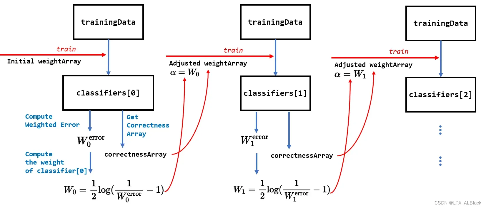
集成过程详见上图,最初我们可以通过基础的权值数组weightArray(所有数据行的权都一样)进行一次基础的树桩分类,得到两个可用于集成的信息:
- 分类器中自我测试下得到分类错误的权值总和\(W_{i}^{\text{error}}\)
- 每一行测试是否正确的布尔数组correctnessArray
继续,定义分类器的权值计算公式:\[ W_{i} = \frac{1}{2} \log(\frac{1}{W_{i}^\text{error}} -1) \tag{2}\] 通过这个公式,我们可以进一步计算出当前分类器的权。同时可以了解到,当一个分类器错误的权重越大,那么本身这个分类器的权就越小
然后,进一步确立一个定义:之前公式1中定义的影响因子\(\alpha\)=\(W_{i}\)。
这个定义成功将上一个分类器的结果同下一个分类器串联了起来,结合公式2的红色总结,再结合公式1中指数函数左右半轴的速度差异性关系,可以得出结论:上一个分类器错误得越多,那么它的权就越小,他对于之后分类器中每个数据行的权值增幅影响也就越小。
总的来说,通过上一个分类计算得到的总权\(W_{i}\)从而影响下一个分类器的权值分配数组,从而影响下一个分类的模型学习过程。
随着这个过程的不断迭代,我们集成器中承载的分类器越来越多,按照AdaBoost的理论,这个时候整体的分类的准确性会不断提高。这时我们就要考虑一个问题,什么时候收敛?下列有几个策略:
- 数目优先原则:我们为集成器设置一个分类器上限,不管当前的集成器的识别率达到到了何种程度,只要数目达到我们要求的上限,那么就自动停下来,确定当前的集成器为最终集成器,不再迭代分类器进行学习。(若前几个少量的分类器就达标了,后续的计算只会浪费开销)
- 识别率优先原则:我们不在意设置多少分类器,只是在意集成器是否达到我们所要求的识别率阈值。一旦达到了阈值便停止当前分类。(若设置的识别率过高,可能导致学习过程过长,甚至可能永远无法实现)
- 混合:顾名思义,设置两个阈值,一个是分类器的数目阈值,一个识别率阈值,任何一个达标便结束集成器构建。
我们代码用的是第三个,这个靠谱一些,能避免前两者的缺陷。
但是这里引入了一个关于集成器的一个非常有意思的讨论话题,就是假如说,若我的集成器通过\(N\)此分类器的组合已经得到了一个相对100%的识别率,那么我们还学习吗?其实这个时候继续学习是可行的,继续学习能进一步扩展集成器的稳定性,保证了下一次类似数据也能保证客观的识别率。(我们会在最后用数据证明这句话的!)
综上,我们可以给出实现代码(细节就不再赘述,可结合上面的图深入理解代码):
	/**
	 ******************
	 * Train the booster.
	 *
	 * @see algorithm.StumpClassifier#train()
	 ******************
	 */
	public void train() {
		// Step 1. Initialize.
		WeightedInstances tempWeightedInstances = null;
		double tempError;
		numClassifiers = 0;

		// Step 2. Build other classifiers.
		for (int i = 0; i < classifiers.length; i++) {
			// Step 2.1 Key code: Construct or adjust the weightedInstances
			if (i == 0) {
				tempWeightedInstances = new WeightedInstances(trainingData);
			} else {
				// Adjust the weights of the data.
				tempWeightedInstances.adjustWeights(classifiers[i - 1].computeCorrectnessArray(),
						classifierWeights[i - 1]);
			} // Of if

			// Step 2.2 Train the next classifier.
			classifiers[i] = new StumpClassifier(tempWeightedInstances);
			classifiers[i].train();

			tempError = classifiers[i].computeWeightedError();

			// Key code: Set the classifier weight.
			classifierWeights[i] = 0.5 * Math.log(1 / tempError - 1);
			if (classifierWeights[i] < 1e-6) {
				classifierWeights[i] = 0;
			} // Of if

			System.out.println("Classifier #" + i + " , weighted error = " + tempError + ", weight = "
					+ classifierWeights[i] + "\r\n");

			numClassifiers++;

			// The accuracy is enough.
			if (stopAfterConverge) {
				double tempTrainingAccuracy = computeTrainingAccuray();
				System.out.println("The accuracy of the booster is: " + tempTrainingAccuracy + "\r\n");
				if (tempTrainingAccuracy > 0.999999) {
					System.out.println("Stop at the round: " + i + " due to converge.\r\n");
					break;
				} // Of if
			} // Of if
		} // Of for i
	}// Of train
(31~35行)代码中要注意的地方就是在计算某个分类器的权\(W_{i}\)时一旦得到的结果超过浮点型的界限,我们可以认定其权为0,通过公式1可以知道,这时迭代的下一个分类器的权值数组是不会有任何变化的(因为增益效果为原来的权值*1.0),即认为这个分类器对于最终我们集成器的贡献为0。
(42~50行)本代码因为采用第三种收敛策略,故外层设置了分类器的个数的循环,但是在代码中留有了识别率达到要求的早熟退出出口。这里computeTrainingAccuray( )函数的思想将在下面介绍。
5.3 并行设计(分类与准确度)思想与代码
要明白集成器是如何计算准确度的,我们首先就要了解到集成器对于任何一条数据进行分类的策略,简单可以用下面个图表示:
首先我们学习得到了一个具有\(n\)个桩分类器的集成器:
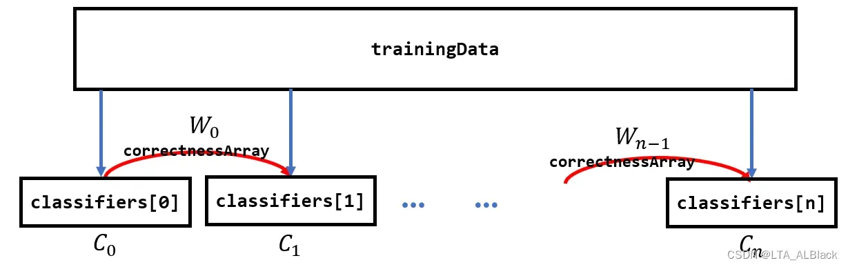
然后已知一个测试用的数据行testingInstance,将这个数据行分别同每个树桩分类器进行测试(细节见4.3:树桩分类器对于测试数据的测试),测试得到了一个预测的标签。
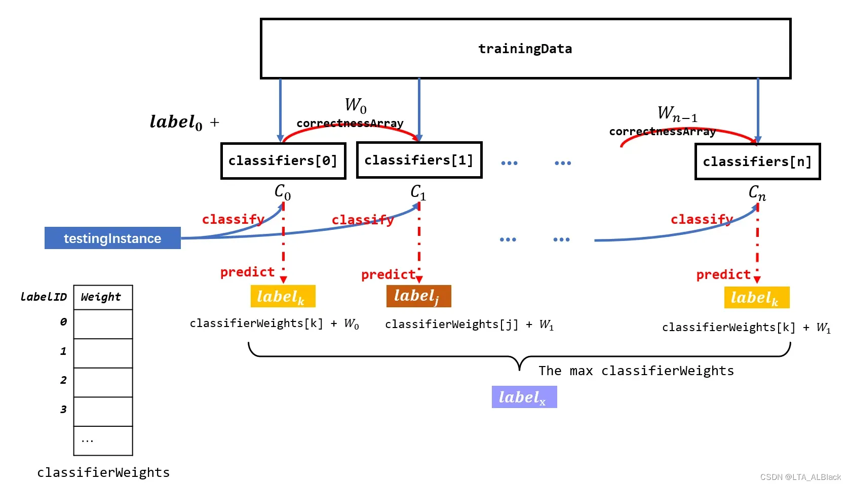
现有一个名为classifierWeights的一维结构,我们将用其作为投票用的一个桶结构。testingInstance基于每个树桩分类器分类得到一个预测标签,鉴定有一个预测标签ID的值为k,便对结构classifierWeights[k]进行加权,而加的权值就是当前分类器的权。
最后判断classifierWeights的最大值并返回其下标,即投票选出权值统计最大的标签。
这个过程的代码描述如下:
	/**
	 ******************
	 * Classify an instance.
	 *
	 * @param paraInstance
	 *            The given instance.
	 * @return The predicted label.
	 ******************
	 */
	public int classify(Instance paraInstance) {
		double[] tempLabelsCountArray = new double[trainingData.classAttribute().numValues()];
		for (int i = 0; i < numClassifiers; i++) {
			int tempLabel = classifiers[i].classify(paraInstance);
			tempLabelsCountArray[tempLabel] += classifierWeights[i];
		} // Of for i

		int resultLabel = -1;
		double tempMax = -1;
		for (int i = 0; i < tempLabelsCountArray.length; i++) {
			if (tempMax < tempLabelsCountArray[i]) {
				tempMax = tempLabelsCountArray[i];
				resultLabel = i;
			} // Of if
		} // Of for

		return resultLabel;
	}// Of classify
由此,准确度的代码便不难得出了:
下面这个计算准确度是用训练了AdaBoost模型的训练集作为测试样本,自己测试自己
	/**
	 ******************
	 * Compute the training accuracy of the booster. It is not weighted.
	 *
	 * @return The training accuracy.
	 ******************
	 */
	public double computeTrainingAccuray() {
		double tempCorrect = 0;

		for (int i = 0; i < trainingData.numInstances(); i++) {
			if (classify(trainingData.instance(i)) == (int) trainingData.instance(i).classValue()) {
				tempCorrect++;
			} // Of if
		} // Of for i

		double tempAccuracy = tempCorrect / trainingData.numInstances();

		return tempAccuracy;
	}// Of computeTrainingAccuray
为了测试方便,还是专门写了个基于某个测试集的准确度计算代码。
	/**
	 ******************
	 * Test the booster.
	 *
	 * @param paraInstances
	 *            The testing set.
	 * @return The classification accuracy.
	 ******************
	 */
	public double test(Instances paraInstances) {
		double tempCorrect = 0;
		paraInstances.setClassIndex(paraInstances.numAttributes() - 1);

		for (int i = 0; i < paraInstances.numInstances(); i++) {
			Instance tempInstance = paraInstances.instance(i);
			if (classify(tempInstance) == (int) tempInstance.classValue()) {
				tempCorrect++;
			} // Of if
		} // Of for i

		double resultAccuracy = tempCorrect / paraInstances.numInstances();
		System.out.println("The accuracy is: " + resultAccuracy);

		return resultAccuracy;
	} // Of test
六、AdaBoost运行效果测试
    /**
	 ******************
	 * For integration test.
	 *
	 * @param args
	 *            Not provided.
	 ******************
	 */
	public static void main(String args[]) {
		System.out.println("Starting AdaBoosting...");
		Booster tempBooster = new Booster("D:/Java DataSet/iris.arff");
		// Booster tempBooster = new Booster("src/data/smalliris.arff");

		tempBooster.setNumBaseClassifiers(100);
		tempBooster.train();

		System.out.println("The training accuracy is: " + tempBooster.computeTrainingAccuray());
	}// Of main
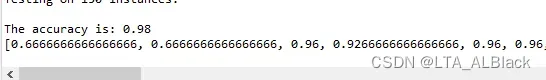
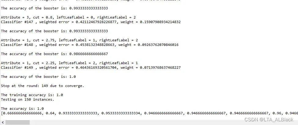
其运行结果如下:
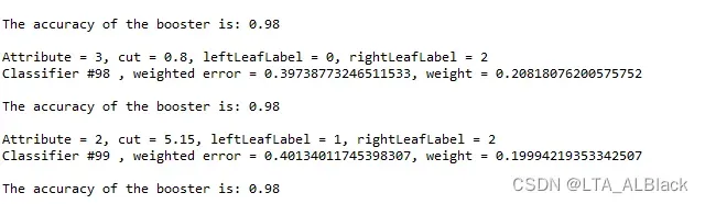
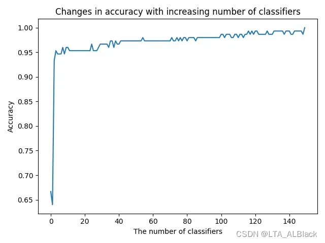
这个结果是对于自身测试所得到的结果,最终的测试效果能达到0.98。不妨想想在4.3的时候单独测试树桩分类器的时候,其识别率只在0.56~0.67区间内,但是通过若干分类器的集成,最终竟然可以直逼0.98的识别率,可谓是“ 三个诸葛亮,定个臭皮匠 ”了。下面给出不同分类器个数反映的识别度变化情况:
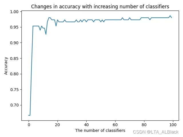
可以发现,其实在非常少的分类器的控制下,相似度已经能达到一个非常高的水准了,大概是在第三个分类器的时候,这种跳变就发生了:
只不过在分类器比较少的时候,整体AdaBoost的识别率非常不稳定,这也是为什么刚刚我们在提出“ 在识别率已经满足我们需要的高度时,是否还需要继续添加分类器 ”时给出了肯定的答案:正是为了提高识别率的稳定性!如上图在超过20的分类器时,全局的识别率非常稳定。
后续当我们将AdaBoost的分类器上限改成200再跑的时候发现数据到150就结束呢,因为在第150个分类器设置之后,第一个100%准确度的样例出现了,检测阈值发现了超过0.99999的准确度,程序提前结束。
通过多次测试可以肯定,基本上最好在130多个分离器或者最差180多个分类器时,此数据的AdaBoost算法能首次出现1.0的识别率。这也侧面证明了AdaBoost在确定识别率方面并不是稳定的,自然,那么最终出现了1.0的识别率也不是一个稳定的状态。
下面我将识别率达到阈值提前结束的限制取消,然后将数目提升到200和500分别测试:
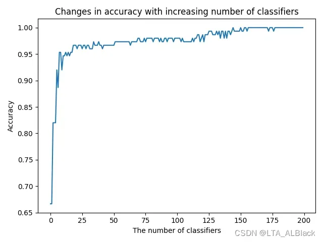
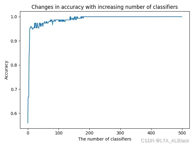
虽然早在200之前,识别率就已经有1.0的情况了,但是这段数据不算稳定,甚至在基本稳定于1.0时的后续仍然有低于1.0的情况。最终当我们将分类设置得足够多时,数据最终稳定了下来。所以对于AdaBoost来说,识别得到1.0也不应当是终点,我们还能继续学习提高稳定度!
(后续关于AdaBoost的内容会继续在本博客中补充)
文章出处登录后可见!