用1层隐藏层的神经网络分类二维数据
现在是时候建立你的第一个神经网络了,它将具有一层隐藏层。你将看到此模型与你使用逻辑回归实现的模型之间的巨大差异。
你将学到如何:
- 实现具有单个隐藏层的2分类神经网络
- 使用具有非线性激活函数的神经元,例如tanh
- 计算交叉熵损失
- 实现前向和后向传播
1- 安装包
让我们首先导入在作业过程中需要的所有软件包。
- numpy是Python科学计算的基本包。
- sklearn提供了用于数据挖掘和分析的简单有效的工具。
- matplotlib 是在Python中常用的绘制图形的库。
- testCases提供了一些测试示例用以评估函数的正确性
- planar_utils提供了此作业中使用的各种函数
import numpy as np
import matplotlib.pyplot as plt
from testCases import *
import sklearn
import sklearn.datasets
import sklearn.linear_model
from planar_utils import plot_decision_boundary, sigmoid, load_planar_dataset, load_extra_datasets

%matplotlib inline

np.random.seed(1)
2- 数据集
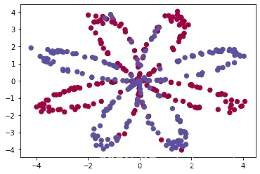
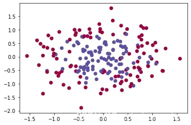
首先,让我们获取处理的数据集。以下代码会将”flower”2分类数据集加载到变量X和Y中。
X, Y = load_planar_dataset()
使用matplotlib可视化数据集。 数据看起来像是带有一些红色(标签y = 0)和一些蓝色(y = 1)点的“花”。 我们的目标是建立一个适合该数据的分类模型。
plt.scatter(X[0, :], X[1, :], c = Y.reshape(X[0, :].shape), s = 40, cmap = plt.cm.Spectral)
<matplotlib.collections.PathCollection at 0x1f9003a74e0>
现在你有:
- 包含特征(x1, x2)的numpy数组(矩阵)X
- 包含标签(红色:0,蓝色:1)的numpy数组(向量)Y。
首先让我们深入地了解一下我们的数据。
练习:数据集中有多少个训练示例?另外,变量X和Y的shape是什么?
提示:如何获得numpy数组的shape维度?
shape_X = X.shape
shape_Y = Y.shape

m = shape_X[1] # 训练数据集大小

print ('The shape of X is: ' + str(shape_X))
print ('The shape of Y is: ' + str(shape_Y))
print ('I have m = %d training examples!' % (m))
The shape of X is: (2, 400)
The shape of Y is: (1, 400)
I have m = 400 training examples!
3- 简单Logistic回归
在构建完整的神经网络之前,首先让我们看看逻辑回归在此问题上的表现。 你可以使用sklearn的内置函数来执行此操作。 运行以下代码以在数据集上训练逻辑回归分类器。
clf = sklearn.linear_model.LogisticRegressionCV()
clf.fit(X.T, Y.T)
d:\vr\virtual_environment\lib\site-packages\sklearn\utils\validation.py:993: DataConversionWarning: A column-vector y was passed when a 1d array was expected. Please change the shape of y to (n_samples, ), for example using ravel().
  y = column_or_1d(y, warn=True)


LogisticRegressionCV()
现在,你可以运行下面的代码以绘制此模型的决策边界:
plot_decision_boundary(lambda x:clf.predict(x), X, Y)
plt.title("Logistic Regression")

LR_predictions = clf.predict(X.T)
print ('Accuracy of logistic regression: %d ' % float((np.dot(Y,LR_predictions) + np.dot(1-Y,1-LR_predictions))/float(Y.size)*100) +
       '% ' + "(percentage of correctly labelled datapoints)")
Accuracy of logistic regression: 47 % (percentage of correctly labelled datapoints)

4- 神经网络模型
从上面我们可以得知Logistic回归不适用于“flower数据集”。现在你将训练带有单个隐藏层的神经网络。
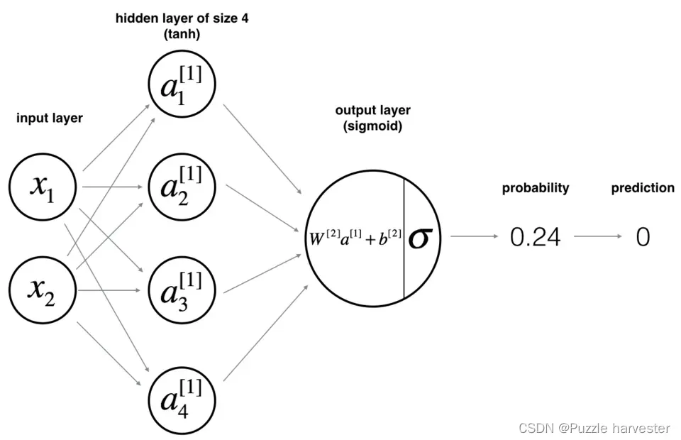
这是我们的模型:
数学原理:
例如:
根据所有的预测数据,你还可以如下计算损失:
提示:
建立神经网络的一般方法是:
- 定义神经网络结构(输入单元数,隐藏单元数等)。
- 初始化模型的参数
- 循环:
- 实现前向传播
- 计算损失
- 后向传播以获得梯度
- 更新参数(梯度下降)
我们通常会构建辅助函数来计算第1-3步,然后将他们合并为nn_model()函数。一旦构建了nn_model()并学习了正确的参数,就可以对新数据进行预测。
4.1- 定义神经网络结构
练习:定义三个变量:
- n_x:输入层的大小
- n_h:隐藏层的大小(将其设置为4)
- n_y:输出层的大小
提示:使用shape来找到n_x和n_y。另外,将隐藏层大小硬编码为4。
def layer_sizes(X, Y):
    n_x = X.shape[0]
    n_h = 4
    n_y = Y.shape[0]

    return (n_x, n_h, n_y)
X_assess, Y_assess = layer_sizes_test_case()
(n_x, n_h, n_y) = layer_sizes(X_assess, Y_assess)
print("The size of the input layer is: n_x = " + str(n_x))
print("The size of the hidden layer is: n_h = " + str(n_h))
print("The size of the output layer is: n_y = " + str(n_y))
The size of the input layer is: n_x = 5
The size of the hidden layer is: n_h = 4
The size of the output layer is: n_y = 2
4.2- 初始化模型的参数
练习:实现函数 initialize_parameters()。
说明:
- 请确保参数大小正确。 如果需要,也可参考上面的神经网络图。
- 使用随机值初始化权重矩阵。
- 使用:np.random.randn(a,b)* 0.01随机初始化维度为(a,b)的矩阵。
- 将偏差向量初始化为零。
- 使用:np.zeros((a,b)) 初始化维度为(a,b)零的矩阵。
def initialize_parameters(n_x, n_h, n_y):
    np.random.seed(2)

    W1 = np.random.randn(n_h, n_x) * 0.01
    b1 = np.zeros((n_h, 1))
    W2 = np.random.randn(n_y, n_h) * 0.01
    b2 = np.zeros((n_y, 1))

    assert (W1.shape == (n_h, n_x))
    assert (b1.shape == (n_h, 1))
    assert (W2.shape == (n_y, n_h))
    assert (b2.shape == (n_y, 1))

    parameters = {"W1": W1,
                  "b1": b1,
                  "W2": W2,
                  "b2": b2}

    return parameters
n_x, n_h, n_y = initialize_parameters_test_case()

parameters = initialize_parameters(n_x, n_h, n_y)
print("W1 = " + str(parameters["W1"]))
print("b1 = " + str(parameters["b1"]))
print("W2 = " + str(parameters["W2"]))
print("b2 = " + str(parameters["b2"]))
W1 = [[-0.00416758 -0.00056267]
 [-0.02136196  0.01640271]
 [-0.01793436 -0.00841747]
 [ 0.00502881 -0.01245288]]
b1 = [[0.]
 [0.]
 [0.]
 [0.]]
W2 = [[-0.01057952 -0.00909008  0.00551454  0.02292208]]
b2 = [[0.]]
4.3- 循环
问题:实现forward_propagation()。
说明:
- 在上方查看分类器的数学表示形式。
- 你可以使用内置在笔记本中的sigmoid()函数。
- 你也可以使用numpy库中的np.tanh()函数。
- 必须执行以下步骤:
- 使用parameters [“ …”]从字典“ parameters”(这是initialize_parameters()的输出)中检索出每个参数。
- 实现正向传播,计算
,
,
和
(所有训练数据的预测结果向量)。
向后传播所需的值存储在cache中, cache将作为反向传播函数的输入。
def forward_propagation(X, parameters):
    """
    参数:
    X -- 输入数据大小(n_x, m)
    parameters -- 包含参数的Python字典(初始化函数的输出)

    返回值:
    A2 -- 用的是sigmoid函数作为输出层的激活函数
    cache -- 包含“Z1”、“A1”、“Z2”和“A2”的字典
    """

    W1 = parameters["W1"]
    b1 = parameters["b1"]
    W2 = parameters["W2"]
    b2 = parameters["b2"]

    Z1 = np.dot(W1, X) + b1
    A1 = np.tanh(Z1)
    Z2 = np.dot(W2, A1) + b2
    A2 = sigmoid(Z2)

    assert(A2.shape == (1, X.shape[1]))

    cache = {"Z1": Z1,
             "A1": A1,
             "Z2": Z2,
             "A2": A2}

    return A2, cache
X_assess, parameters = forward_propagation_test_case()

A2, cache = forward_propagation(X_assess, parameters)

print(np.mean(cache['Z1']) ,np.mean(cache['A1']),np.mean(cache['Z2']),np.mean(cache['A2']))
-0.0004997557777419913 -0.0004969633532317802 0.0004381874509591466 0.500109546852431
现在,你已经计算了包含每个示例的的
(在Python变量”A2″中),其中,你可以计算损失函数如下:
练习:实现compute_cost()以计算损失的值。
说明:
- 有很多种方法可以实现交叉熵损失。 我们为你提供了实现方法:
:
logprobs = np.multiply(np.log(A2),Y)
cost = - np.sum(logprobs)                # no need to use a for loop!
(你也可以使用np.multiply()然后使用np.sum()或直接使用np.dot())。
def compute_cost(A2, Y, parameters):

    m = Y.shape[1]

    logprobs = Y * np.log(A2) + (1 - Y) * np.log(1 - A2)
    cost = -1 / m * np.sum(logprobs)

    cost = np.squeeze(cost)

    assert(isinstance(cost, float))
    return cost
A2, Y_assess, parameters = compute_cost_test_case()

print("cost = " + str(compute_cost(A2, Y_assess, parameters)))
cost = 0.6929198937761265
现在,通过使用正向传播期间计算的缓存,你可以实现后向传播。
问题:实现函数backward_propagation()。
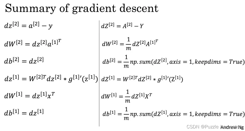
说明:反向传播通常是深度学习中最难(最数学)的部分。为了帮助你更好地了解,我们提供了反向传播课程的幻灯片。你将要使用此幻灯片右侧的六个方程式以构建向量化实现。
- 请注意, 表示元素乘法。
- 你将使用在深度学习中很常见的编码表示方法:
- dW1 =
- db1 =
- dW2 =
- db2 =
- dW1 =
- 提示:
- 要计算dZ1,你首先需要计算
。由于
是tanh激活函数,因此如果
则
。所以你可以使用
(1 - np.power(A1, 2))计算
- 要计算dZ1,你首先需要计算
def backward_propagation(parameters, cache, X, Y):
    """
    参数:
        parameters -- 包含参数的Python字典
        cache -- 包含“Z1”、“A1”、“Z2”和“A2”的字典。
        X -- 输入数据大小(2, 样例数)
        Y -- “true”标签的形状向量(1, 样例数)
    返回值:
        grads -- 包含不同参数梯度的Python字典
    """

    W1 = parameters["W1"]
    W2 = parameters["W2"]

    A1 = cache["A1"]
    A2 = cache["A2"]

    dZ2 = A2 - Y
    dW2 = 1 / m * np.dot(dZ2, A1.T)
    db2 = 1 / m * np.sum(dZ2, axis = 1, keepdims = True)
    dZ1 = np.dot(W2.T, dZ2) * (1 - np.power(A1, 2))
    dW1 = 1 / m * np.dot(dZ1, X.T)
    db1 = 1 / m * np.sum(dZ1, axis = 1, keepdims = True)


    grads = {"dW1": dW1,
             "db1": db1,
             "dW2": dW2,
             "db2": db2}

    return grads
parameters, cache, X_assess, Y_assess = backward_propagation_test_case()

grads = backward_propagation(parameters, cache, X_assess, Y_assess)
print ("dW1 = "+ str(grads["dW1"]))
print ("db1 = "+ str(grads["db1"]))
print ("dW2 = "+ str(grads["dW2"]))
print ("db2 = "+ str(grads["db2"]))
dW1 = [[ 7.64031222e-05 -5.31526069e-05]
 [ 6.55085623e-05 -4.55760073e-05]
 [-3.98134983e-05  2.77034561e-05]
 [-1.65477342e-04  1.15134485e-04]]
db1 = [[-5.22957353e-06]
 [-4.54546847e-06]
 [ 2.72996662e-06]
 [ 1.13405247e-05]]
dW2 = [[ 2.72709941e-05  2.36520302e-04  8.72185240e-05 -9.88737100e-05]]
db2 = [[0.00049421]]
问题:实现参数更新。 使用梯度下降,你必须使用(dW1,db1,dW2,db2)才能更新(W1,b1,W2,b2)。
一般的梯度下降规则:$ \theta = \theta – \alpha \frac{\partial J }{ \partial \theta }\alpha
\theta$代表一个参数。
图示:具有良好的学习速率(收敛)和较差的学习速率(发散)的梯度下降算法。

def update_parameters(parameters, grads, learning_rate = 1.2):

    W1 = parameters["W1"]
    b1 = parameters["b1"]
    W2 = parameters["W2"]
    b2 = parameters["b2"]

    dW1 = grads["dW1"]
    db1 = grads["db1"]
    dW2 = grads["dW2"]
    db2 = grads["db2"]

    W1 = W1 - learning_rate * dW1
    b1 = b1 - learning_rate * db1
    W2 = W2 - learning_rate * dW2
    b2 = b2 - learning_rate * db2

    parameters = {"W1": W1,
                  "b1": b1,
                  "W2": W2,
                  "b2": b2}

    return parameters
parameters, grads = update_parameters_test_case()
parameters = update_parameters(parameters, grads)

print("W1 = " + str(parameters["W1"]))
print("b1 = " + str(parameters["b1"]))
print("W2 = " + str(parameters["W2"]))
print("b2 = " + str(parameters["b2"]))
W1 = [[-0.00643025  0.01936718]
 [-0.02410458  0.03978052]
 [-0.01653973 -0.02096177]
 [ 0.01046864 -0.05990141]]
b1 = [[-1.02420756e-06]
 [ 1.27373948e-05]
 [ 8.32996807e-07]
 [-3.20136836e-06]]
W2 = [[-0.01041081 -0.04463285  0.01758031  0.04747113]]
b2 = [[0.00010457]]
4.4- 在nn_model()中集成4.1、4.2和4.3部分中的函数
问题:在nn_model()中建立你的神经网络模型。
说明:神经网络模型必须正确的顺序组合先前构建的函数。
def nn_model(X, Y, n_h, num_iterations = 10000, print_cost = False):
    np.random.seed(3)

    n_x = layer_sizes(X, Y)[0]
    n_y = layer_sizes(X, Y)[2]

    parameters = initialize_parameters(n_x, n_h, n_y)
    W1 = parameters["W1"]
    b1 = parameters["b1"]
    W2 = parameters["W2"]
    b2 = parameters["b2"]

    for i in range(0, num_iterations):

        A2, cache = forward_propagation(X, parameters)

        cost = compute_cost(A2, Y, parameters)

        grads = backward_propagation(parameters, cache, X, Y)

        parameters = update_parameters(parameters, grads)

        if print_cost and i % 1000 == 0:
            print ("Cost after iteration %i: %f" %(i, cost))
    return parameters
X_assess, Y_assess = nn_model_test_case()

parameters = nn_model(X_assess, Y_assess, 4, num_iterations=10000, print_cost=False)
print("W1 = " + str(parameters["W1"]))
print("b1 = " + str(parameters["b1"]))
print("W2 = " + str(parameters["W2"]))
print("b2 = " + str(parameters["b2"]))
d:\vr\virtual_environment\lib\site-packages\ipykernel_launcher.py:5: RuntimeWarning: divide by zero encountered in log
  """


W1 = [[-2.83554662  1.72205388]
 [-3.37802227  0.92947318]
 [-2.54331167  2.02087066]
 [ 3.37518445 -0.93029167]]
b1 = [[ 1.3407194 ]
 [ 1.67353851]
 [ 1.23099392]
 [-1.67347162]]
W2 = [[-43.10905352 -43.84863143 -42.31070324  43.80751756]]
b2 = [[-0.93568323]]
4.5- 预测
问题:使用你的模型通过构建predict()函数进行预测。
使用正向传播来预测结果。
提示:predictions =
例如,如果你想基于阈值将矩阵X设为0和1,则可以执行以下操作: X_new = (X > threshold)
round()函数:
一般该函数遵循四舍五入原则,但是需要特别注意的是,当整数部分以0结束时,round函数一律是向下取整。
def predict(parameters, X):

    A2, cache = forward_propagation(X, parameters)
    predictions = np.round(A2)

    return predictions
parameters, X_assess = predict_test_case()

predictions = predict(parameters, X_assess)
print("predictions mean = " + str(np.mean(predictions)))
predictions mean = 0.6666666666666666
现在运行模型以查看其如何在二维数据集上运行。运行以下代码以使用含有隐藏单元的单个隐藏层测试模型。
parameters = nn_model(X, Y, n_h = 4, num_iterations = 10000, print_cost=True)
plot_decision_boundary(lambda x: predict(parameters, x.T), X, Y)
plt.title("Decision Boundary for hidden layer size " + str(4))
Cost after iteration 0: 0.693048
Cost after iteration 1000: 0.288083
Cost after iteration 2000: 0.254385
Cost after iteration 3000: 0.233864
Cost after iteration 4000: 0.226792
Cost after iteration 5000: 0.222644
Cost after iteration 6000: 0.219731
Cost after iteration 7000: 0.217504
Cost after iteration 8000: 0.219440
Cost after iteration 9000: 0.218553


Text(0.5, 1.0, 'Decision Boundary for hidden layer size 4')

predictions = predict(parameters, X)
print ('Accuracy: %d' % float((np.dot(Y,predictions.T) + np.dot(1-Y,1-predictions.T))/float(Y.size)*100) + '%')
Accuracy: 90%
与Logistic回归相比,准确性确实更高。 该模型学习了flower的叶子图案! 与逻辑回归不同,神经网络甚至能够学习非线性的决策边界。
现在,让我们尝试几种不同的隐藏层大小。
4.6- 调整隐藏层大小
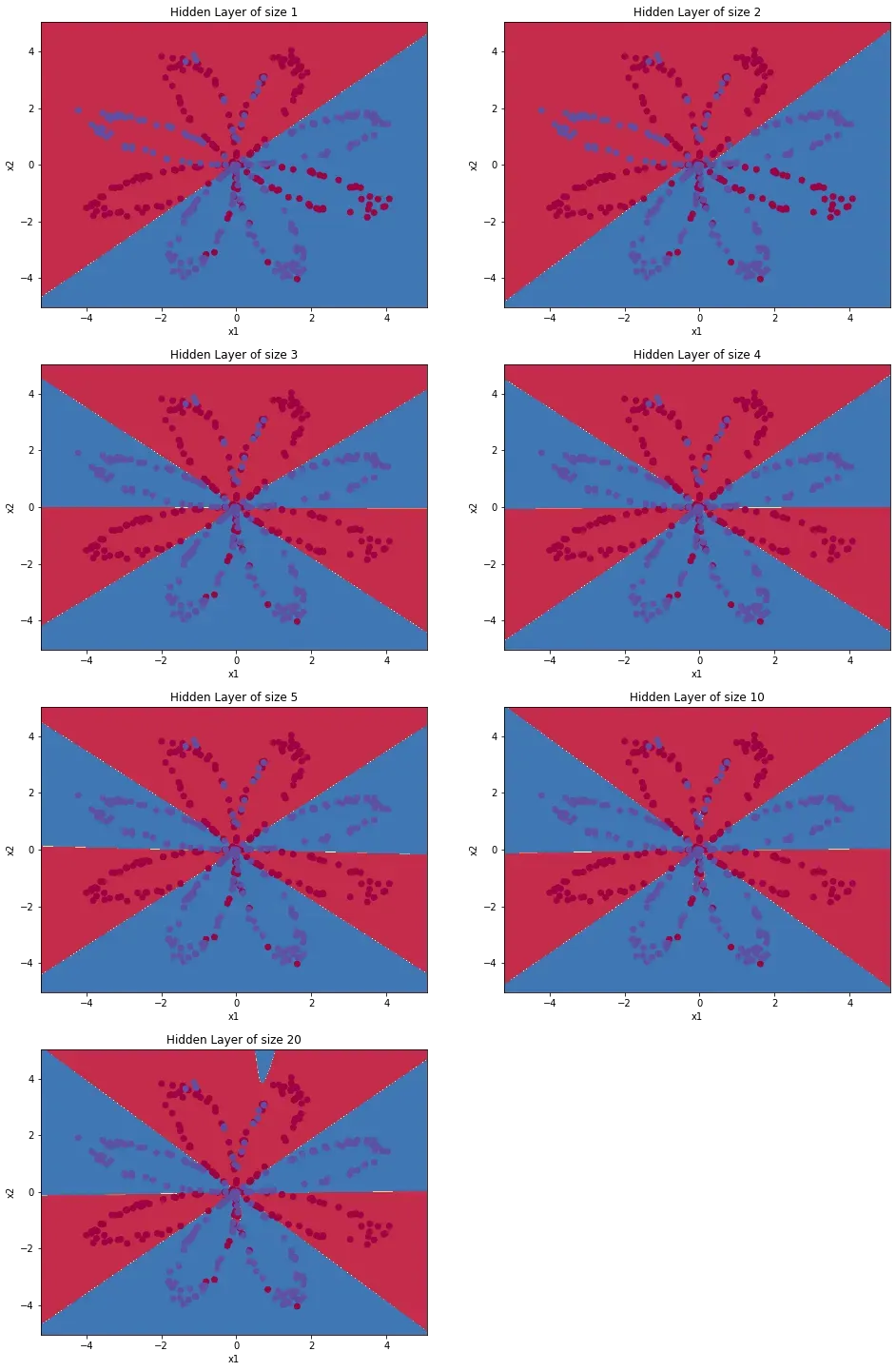
运行以下代码(可能需要1-2分钟), 你将观察到不同大小隐藏层的模型的不同表现。
plt.figure(figsize=(16, 32))
hidden_layer_sizes = [1, 2, 3, 4, 5, 10, 20]
for i, n_h in enumerate(hidden_layer_sizes):
    plt.subplot(5, 2, i+1)
    plt.title('Hidden Layer of size %d' % n_h)
    parameters = nn_model(X, Y, n_h, num_iterations = 5000)
    plot_decision_boundary(lambda x: predict(parameters, x.T), X, Y)
    predictions = predict(parameters, X)
    accuracy = float((np.dot(Y,predictions.T) + np.dot(1-Y,1-predictions.T))/float(Y.size)*100)
    print ("Accuracy for {} hidden units: {} %".format(n_h, accuracy))
Accuracy for 1 hidden units: 67.5 %
Accuracy for 2 hidden units: 67.25 %
Accuracy for 3 hidden units: 90.75 %
Accuracy for 4 hidden units: 90.5 %
Accuracy for 5 hidden units: 91.25 %
Accuracy for 10 hidden units: 90.25 %
Accuracy for 20 hidden units: 90.5 %
说明:
- 较大的模型(具有更多隐藏的单元)能够更好地拟合训练集,直到最终最大的模型过拟合数据为止。
- 隐藏层的最佳大小似乎在n_h = 5左右。的确,此值似乎很好地拟合了数据,而又不会引起明显的过度拟合。
- 稍后你还将学习正则化,帮助构建更大的模型(例如n_h = 50)而不会过度拟合。
总结:
- 建立具有隐藏层的完整神经网络
- 善用非线性单位
- 实现正向传播和反向传播,并训练神经网络
- 了解不同隐藏层大小(包括过度拟合)的影响。
5- 模型在其他数据集上的性能
noisy_circles, noisy_moons, blobs, gaussian_quantiles, no_structure = load_extra_datasets()
datasets = {"noisy_circles": noisy_circles,
            "noisy_moons": noisy_moons,
            "blobs": blobs,
            "gaussian_quantiles": gaussian_quantiles}

dataset = "noisy_circles"

X, Y = datasets[dataset]
X, Y = X.T, Y.reshape(1, Y.shape[0])

if dataset == "blobs":
    Y = Y%2

plt.scatter(X[0, :], X[1, :], c=Y.reshape(X[0,:].shape), s=40, cmap=plt.cm.Spectral);
文章出处登录后可见!