单通道、多通道图像读取
单通道图
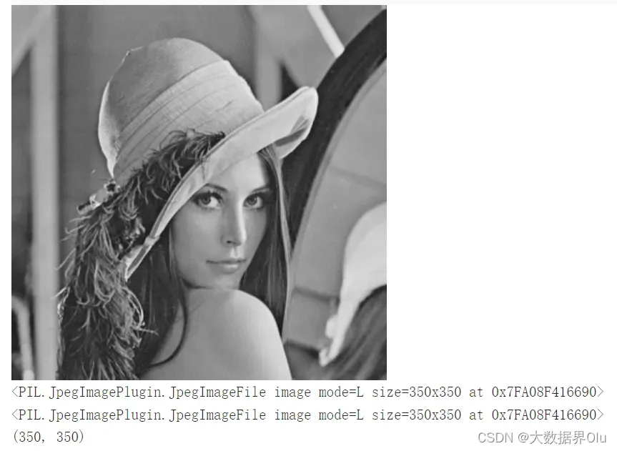
俗称灰度图,每个像素点只能有有一个值表示颜色,它的像素值在0到255之间,0是黑色,255是白色,中间值是一些不同等级的灰色。
import numpy as np
import cv2
import matplotlib.pyplot as plt
import paddle
from PIL import Image
img = Image.open('lena-gray.jpg')

display(img)
print(img)
print(img.size)
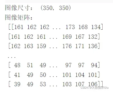
# 将图片转为矩阵表示
img_np = np.array(img)
print("图像尺寸:", img_np.shape)
print("图像矩阵:\n", img_np)
# 不妨把上面的矩阵保存成txt,但是如果直接保存,会变成科学计数法,查看一下np.savetxt()的用法
# 将矩阵保存成文本,数字格式为整数
# np.savetxt('lena_gray.txt', np.array(img), fmt='%4d')
np.savetxt('lena_gray.txt', img, fmt='%4d')
三通道图
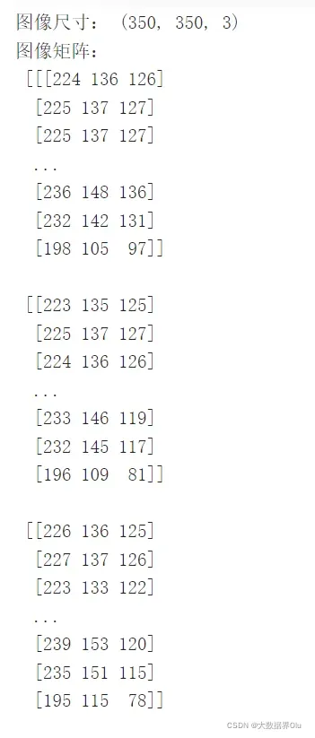
每个像素点都有3个值表示 ,所以就是3通道。也有4通道的图。例如RGB图片即为三通道图片,RGB色彩模式是工业界的一种颜色标准,是通过对红®、绿(G)、蓝(B)三个颜色通道的变化以及它们相互之间的叠加来得到各式各样的颜色的,RGB即是代表红、绿、蓝三个通道的颜色,这个标准几乎包括了人类视力所能感知的所有颜色,是目前运用最广的颜色系统之一。
img = Image.open('lena.jpg')
# 将图片转为矩阵表示
img_np = np.array(img)
print("图像尺寸:", img_np.shape)
print("图像矩阵:\n", img_np)
(三)四通道图
多一个alpha通道,用作不透明参数
通道分离与转换
彩色图的BGR三个通道是可以分开单独访问的,也可以将单独的三个通道合并成一副图像。分别使用cv2.split()和cv2.merge():
# 使用PIL分离颜色通道
r,g,b = img.split()
# 获取r通道转的灰度图
print(r,'\n',g,'\n',b)
print(type(r))
# 获取第一个通道转的灰度图
r = img.getchannel(0)
# 获取第二个通道转的灰度图
display(img.getchannel(1))
# 获取第二个通道转的灰度图
display(img.getchannel(2))
# 将矩阵保存成文本,数字格式为整数
np.savetxt('lena-r.txt', r, fmt='%4d')
np.savetxt('lena-g.txt', g, fmt='%4d')
np.savetxt('lena-b.txt', b, fmt='%4d')
通道分离与合并
彩色图的BGR三个通道是可以分开单独访问的,也可以将单独的三个通道合并成一副图像。分别使用cv2.split()和cv2.merge():
# 使用PIL分离颜色通道
r,g,b = img.split()
# 获取r通道转的灰度图
print(r,'\n',g,'\n',b)
print(type(r))
# 获取第一个通道转的灰度图
r = img.getchannel(0)
# 获取第二个通道转的灰度图
display(img.getchannel(1))

# 获取b通道转的灰度图
b
# 将矩阵保存成文本,数字格式为整数
np.savetxt('lena-r.txt', r, fmt='%4d')
np.savetxt('lena-g.txt', g, fmt='%4d')
np.savetxt('lena-b.txt', b, fmt='%4d')
# 引入依赖包
%matplotlib inline
import cv2
import matplotlib.pyplot as plt

img = cv2.imread('lena.jpg')

# 通道分割
b, g, r = cv2.split(img)

# 通道合并
RGB_Image=cv2.merge([b,g,r])
RGB_Image = cv2.cvtColor(RGB_Image, cv2.COLOR_BGR2RGB)
plt.figure(figsize=(12,12))
#显示各通道信息
plt.subplot(141)
plt.imshow(RGB_Image,'gray')
plt.title('RGB_Image')
plt.subplot(142)
plt.imshow(r,'gray')
plt.title('R_Channel')
plt.subplot(143)
plt.imshow(g,'gray')
plt.title('G_Channel')
plt.subplot(144)
plt.imshow(b,'gray')
plt.title('B_Channel')
/opt/conda/envs/python35-paddle120-env/lib/python3.7/site-packages/matplotlib/cbook/__init__.py:2349: DeprecationWarning: Using or importing the ABCs from 'collections' instead of from 'collections.abc' is deprecated, and in 3.8 it will stop working
  if isinstance(obj, collections.Iterator):
/opt/conda/envs/python35-paddle120-env/lib/python3.7/site-packages/matplotlib/cbook/__init__.py:2366: DeprecationWarning: Using or importing the ABCs from 'collections' instead of from 'collections.abc' is deprecated, and in 3.8 it will stop working
  return list(data) if isinstance(data, collections.MappingView) else data
/opt/conda/envs/python35-paddle120-env/lib/python3.7/site-packages/numpy/lib/type_check.py:546: DeprecationWarning: np.asscalar(a) is deprecated since NumPy v1.16, use a.item() instead
  'a.item() instead', DeprecationWarning, stacklevel=1)
颜色空间转换
最常用的颜色空间转换如下:
RGB或BGR到灰度(COLOR_RGB2GRAY,COLOR_BGR2GRAY)
RGB或BGR到YcrCb(或YCC)(COLOR_RGB2YCrCb,COLOR_BGR2YCrCb)
RGB或BGR到HSV(COLOR_RGB2HSV,COLOR_BGR2HSV)
RGB或BGR到Luv(COLOR_RGB2Luv,COLOR_BGR2Luv)
灰度到RGB或BGR(COLOR_GRAY2RGB,COLOR_GRAY2BGR)
颜色转换其实是数学运算,如灰度化最常用的是:gray=R0.299+G0.587+B*0.114。
img = cv2.imread('lena.jpg')
# 转换为灰度图
img_gray = cv2.cvtColor(img, cv2.COLOR_BGR2GRAY)
# 保存灰度图
cv2.imwrite('img_gray.jpg', img_gray)
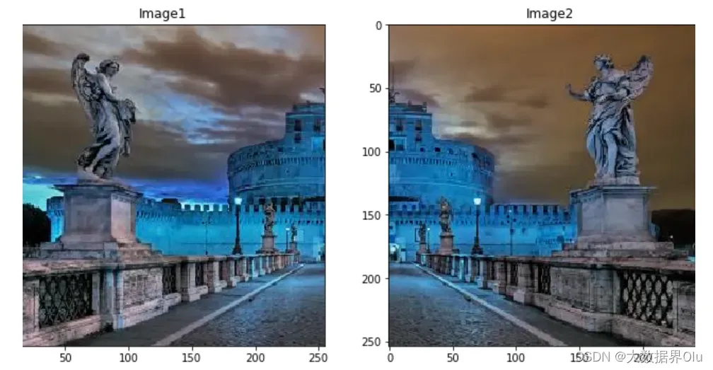
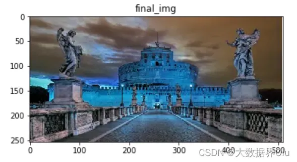
图像拼接与几何变换
拼接
%matplotlib inline
import numpy as np
import cv2
import matplotlib.pyplot as plt

path3 = 'test.jpg'

img3 = cv2.imread(path3)

# the image height
sum_rows = img3.shape[0]
print(img3.shape)
# print(sum_rows)
# the image length
sum_cols = img3.shape[1]
# print(sum_cols)
part1 = img3[0:sum_rows, 0:int(sum_cols/2)]
print(part1.shape)
part2 = img3[0:sum_rows, int(sum_cols/2):sum_cols]
print(part2.shape)

plt.figure(figsize=(12,12))
#显示各通道信息
plt.subplot(121)
plt.imshow(part1)
plt.title('Image1')
plt.subplot(122)
plt.imshow(part2)
plt.title('Image2')
img1 = part1
img2 = part2

# new image
final_matrix = np.zeros((254, 510, 3), np.uint8)
# change
final_matrix[0:254, 0:255] = img1
final_matrix[0:254, 255:510] = img2

plt.subplot(111)
plt.imshow(final_matrix)
plt.title('final_img')
几何变换
实现旋转、平移和缩放图片
OpenCV函数:cv2.resize(), cv2.flip(), cv2.warpAffine()
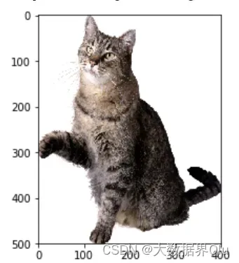
缩放图片
缩放就是调整图片的大小,使用cv2.resize()函数实现缩放。可以按照比例缩放,也可以按照指定的大小缩放: 我们也可以指定缩放方法interpolation,更专业点叫插值方法,默认是INTER_LINEAR
缩放过程中有五种插值方式:
cv2.INTER_NEAREST 最近邻插值
cv2.INTER_LINEAR 线性插值
cv2.INTER_AREA 基于局部像素的重采样,区域插值
cv2.INTER_CUBIC 基于邻域4×4像素的三次插值
cv2.INTER_LANCZOS4 基于8×8像素邻域的Lanczos插值
img = cv2.imread('cat.png')
img = cv2.cvtColor(img, cv2.COLOR_BGR2RGB)
print(img.shape)
# 按照指定的宽度、高度缩放图片
res = cv2.resize(img, (400, 500))
plt.imshow(res)
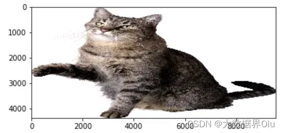
# 按照比例缩放,如x,y轴均放大一倍
res2 = cv2.resize(img, None, fx=5, fy=2, interpolation=cv2.INTER_LINEAR)
plt.imshow(res2)
翻转图片
镜像翻转图片,可以用cv2.flip()函数: 其中,参数2 = 0:垂直翻转(沿x轴),参数2 > 0: 水平翻转(沿y轴),参数2 < 0: 水平垂直翻转。
dst = cv2.flip(img, 1)
plt.imshow(dst)
平移图片
要平移图片,我们需要定义下面这样一个矩阵,tx,ty是向x和y方向平移的距离:
![]()
# 平移图片
import numpy as np
# 获得图片的高、宽
rows, cols = img.shape[:2]

# 定义平移矩阵,需要是numpy的float32类型
# x轴平移200,y轴平移500
M = np.float32([[1, 0, 100], [0, 1, 500]])
# 用仿射变换实现平移
dst = cv2.warpAffine(img, M, (cols, rows))
图像二值化处理
- 使用固定阈值、自适应阈值和Otsu阈值法”二值化”图像
- OpenCV函数:cv2.threshold(), cv2.adaptiveThreshold()
阈值分割
固定阈值分割很直接,一句话说就是像素点值大于阈值变成一类值,小于阈值变成另一类值。
cv2.threshold()用来实现阈值分割,ret是return value缩写,代表当前的阈值。函数有4个参数:
- 参数1:要处理的原图,一般是灰度图
- 参数2:设定的阈值
- 参数3:最大阈值,一般为255
- 参数4:阈值的方式,主要有5种
0: THRESH_BINARY 当前点值大于阈值时,取Maxval,也就是第四个参数,否则设置为0
1: THRESH_BINARY_INV 当前点值大于阈值时,设置为0,否则设置为Maxval
2: THRESH_TRUNC 当前点值大于阈值时,设置为阈值,否则不改变
3: THRESH_TOZERO 当前点值大于阈值时,不改变,否则设置为0
4:THRESH_TOZERO_INV 当前点值大于阈值时,设置为0,否则不改变
import cv2

# 灰度图读入
img = cv2.imread('lena.jpg', 0)
# 颜色通道转换
img = cv2.cvtColor(img, cv2.COLOR_BGR2RGB)
ret, th = cv2.threshold(img, 127, 255, cv2.THRESH_BINARY)
# 阈值分割

plt.imshow(th)
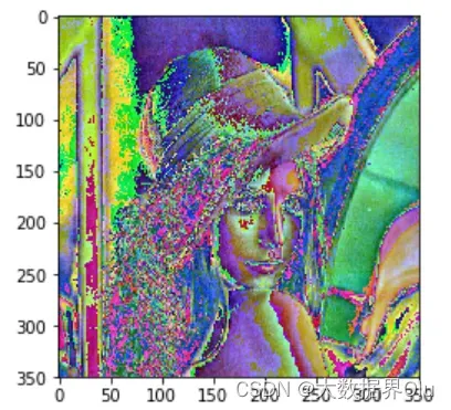
图像归一化处理
数据的标准化是指将数据按照比例缩放,使之落入一个特定的区间。将数据通过去均值,实现中心化。处理后的数据呈正态分布,即均值为零。
# HWC to CHW
# img = img.transpose((2, 0, 1))

#Normalize
# img = img / 255         #像素值归一化
mean = [0.31169346, 0.25506335, 0.12432463]
std = [0.34042713, 0.29819837, 0.1375536]
# img[0] = (img[0] - mean[0]) / std[0]
# img[1] = (img[1] - mean[1]) / std[1]
# img[2] = (img[2] - mean[2]) / std[2]

# print(img[2])
import numpy as np
from PIL import Image
from paddle.vision.transforms import functional as F


img = np.asarray(Image.open('lena.jpg'))

mean = [0.31169346, 0.25506335, 0.12432463]
std = [0.34042713, 0.29819837, 0.1375536]
normalized_img = F.normalize(img, mean, std, data_format='HWC')

normalized_img = Image.fromarray(np.uint8(normalized_img))
plt.imshow(normalized_img)
<matplotlib.image.AxesImage at 0x7fa06029d450>
文章出处登录后可见!