Paper：https://openaccess.thecvf.com/content_iccv_2013/papers/Burgos-Artizzu_Robust_Face_Landmark_2013_ICCV_paper.pdf

Dataset: https://data.caltech.edu/records/20099

动机

在这篇文章中，作者为了解决面部关键点估计时的遮挡和形状的差异问题，提出了一种名为RCPR( Robust Cascaded Pose Regression)的方法，在RCPR方法训练时需要用到每一个关键点是否被遮挡的ground-truth信息，因此作者就以一种较小成本的制作方法在训练集中为每一个landmark 添加了一个 flag 用来编码这个关键点的可见度（visibility）信息。作者将这个添加关键点可见度信息的数据集成为Caltech Occluded Faces in the Wild（COFW）数据集。

本篇博客的重点不在RCPR方法上，读者若感兴趣可以通过上面原文的链接自行了解，下面我们将重点关注数据集的内容和使用方法上。

COFW数据集介绍

为每张图片的关键点添加了是否被遮挡的标注后，可视化效果如下，红色代表被遮挡，绿色代表未遮挡。

可见度信息添加方式其实很简单，就是在原先关键点的标注信息之后，为每个关键点添加第三维度的信息，也就是每个关键点的标注变成了。作者使用RCPR方法对着三个维度同时预测

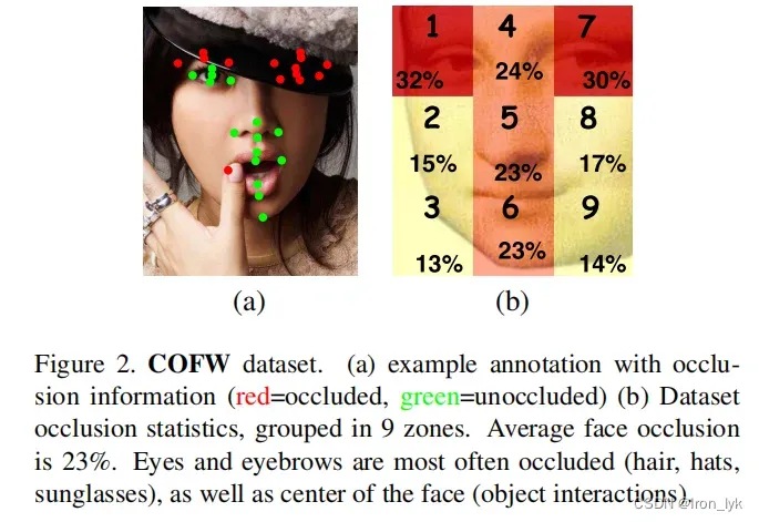
正如名字一样，作者提出COFW数据集的初衷是为了呈现现实世界条件下的人脸，因此COFW数据集中的数据在遮挡和姿态上都更加具有挑战性。COFW数据集共包含1007张images，收集于各种各样的来源，所有的图片被手工标注了与LFPW[1]数据集中一样的29个关键点。数据集中的面部被不同程度的遮挡，平均遮挡率为28%，并且遮挡类型的差异很大。

COFW数据集使用（代码）

通过上面的官方链接下载后，有三个文件：COFW、COFW_color、documentation。

COFW文件夹对应的是灰度数据，COFW_color对应的是RGB数据，documentation是文档的其他相关内容。下面我们主要以COFW文件夹进行讲解。在”./COFW/common/xpburgos/behavior/code/pose/”文件夹下放置了三个文件：COFW_test.mat，COFW_train.mat 和 loadCOFW.m。前两个是存放测试集、训练集数据的mat格式文件。loadCOFW.m是官方给的数据格式及读取说明，下面是对数据格式的介绍。

%Specify files containing training/testing images, load data
trFile='COFW_train.mat';testFile='COFW_test.mat';
load(trFile,'phisTr','IsTr','bboxesTr');
load(testFile,'phisT','IsT','bboxesT');

%% CONTENTS of files
%IsTr = training images = cell(1345,1) 
%IsT = testing images = cell(507,1) 
%phisTr = training ground truth = [1345 x 87]  where 1..29 is X position, 30..58 Y position, 59..87 occlusion bit
%phisT = testing ground truth = [507 x 87]  where 1..29 is X position, 30..58 Y position, 59..87 occlusion bit
%bboxesTr = training face bounding boxes = [1345 x 4]  (left, top, width, height)
%bboxesT = testing face bounding boxes = [507 x 4]  (left, top, width, height)
%

% NOTE 1: First 845 training images belong to LFPW dataset (unoccluded), only remaining 500 images are from COFW
% NOTE 2: Face bounding boxes are not perfect, as they simulate a real face detector

由上可以看出，COFW_test.mat和COFW_train.mat中分别有三个cell：‘phisTr’，’IsTr’，’bboxesTr’。以训练集为例：‘phisTr’的size为[1345, 87]，第一个维度1345表示有1345张图像，其中前845张是来自于LFPW数据集（unoccluded），后500张图像来自COFW数据集，第二个维度87的前29个值表示关键点x坐标，中间29个值表示y坐标，最后29个值表示关键点是否被遮挡（0或1）； ‘IsTr’的size是[1345,1]，表示1345张图片的ref，可以通过它来获取原始图像的数据；‘bboxesTr’的size是[1345,4]，第二个维度4表示每张图片中人脸bounding box 的左上角的(x,y)坐标值以及框的宽和高，（xmin,ymin,weight,height).

下面是使用python对COFW_test.mat文件读取，并显示第二张图片的代码：

import numpy as np
import h5py
import cv2
# import scipy

# test = scipy.io.loadmat("COFW_test.mat")
# 用scio.io.loadmat读取时报错：NotImplementedError: Please use HDF reader for matlab v7.3 files
test = h5py.File('COFW_test.mat',"r")

print(test.keys())        # <KeysViewHDF5 ['#refs#', 'IsT', 'bboxesT', 'phisT']>
print(test["IsT"])        # <HDF5 dataset "IsT": shape (1, 507), type "|O">
print(test["bboxesT"])    # <HDF5 dataset "bboxesT": shape (4, 507), type "<f8">
print(test["phisT"])      # <HDF5 dataset "phisT": shape (87, 507), type "<f8">
print(type(test["IsT"]))  # <class 'h5py._hl.dataset.Dataset'>

images = np.transpose(test['IsT'])  # 所有测试集图像的ref
num = 1                             
img_name = images[num][0]           # 获取第 num 个图像的ref
img = test[img_name]                # 读取第 num 个图像的数据

print(img)                          # <HDF5 dataset "b": shape (239, 179), type "|u1">
print(type(img))                    # <class 'h5py._hl.dataset.Dataset'>

img = np.transpose(test[img_name])  # 转换为np数组，并对维度进行转置

print(type(img))                    # <class 'numpy.ndarray'>
print(img.shape)                    # (179, 239)

cv2.imshow("test_img_0",img)
cv2.waitKey(0)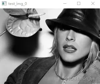

该图片的bbox真实值读取和可视化代码如下：

# 可视化人脸 bounding box
img = np.expand_dims(img,2).repeat(3,2)     # 将img的格式变为（w,h,3），否则cv2.rectangle会报错
print(img.shape)                            # (244, 326, 3)
boxes = test["bboxesT"]
box = boxes[:,num]
print(box)
cv2.rectangle(img, (int(box[0]),int(box[1])), (int(box[0]+box[2]),int(box[1]+box[3])), (0, 0, 255), 2)
cv2.imshow("test_img_0_rect",img)
cv2.waitKey(0)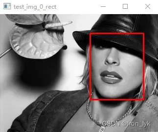

PS：官方文档说给出的人脸bounding boxes可能不是很精确，想使用的小伙伴需谨慎

提取人脸关键点坐标及其能见度，并可视化（红色的点表示被遮挡，绿色的点表示可见），代码如下：

# 可视化关键点及其对应的能见度
ph = np.array(test["phisT"])
x_y_v = ph[:,num]
x = x_y_v[0:29]
y = x_y_v[29:58]
v = x_y_v[58:]
for i in range(len(x)):  
    temp_x, temp_y, temp_v = int(x[i]), int(y[i]), int(v[i])
    if temp_v == 1:
        cv2.circle(img, (int(temp_x),int(temp_y)), 1, (0, 0, 255), 2)
    else:
        cv2.circle(img, (int(temp_x),int(temp_y)), 1, (80, 200, 120), 2)

cv2.imshow("test_img_0_landmark",img)
cv2.waitKey(0)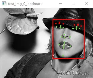

[1] P. Belhumeur, D. Jacobs, D. Kriegman, and N. Kumar. Localizing parts of faces using a concensus of exemplars. In CVPR, 2011.

文章出处登录后可见！

已经登录？立即刷新

COFW数据集介绍以及代码读取

动机

COFW数据集介绍

COFW数据集使用（代码）

相关推荐