DataFrame 是由多种类型的列构成的二维标签数据结构,类似于 Excel 、SQL 表,或 Series 对象构成的字典。DataFrame 是最常用的 Pandas 对象,与 Series 一样,DataFrame 支持多种类型的输入数据:
- 一维 ndarray、列表、字典、Series 字典
- 二维 numpy.ndarray
- 结构多维数组或记录多维数组
SeriesDataFrame
除了数据,还可以有选择地传递 index(行标签)和 columns(列标签)参数。传递了索引或列,就可以确保生成的 DataFrame 里包含索引或列。Series 字典加上指定索引时,会丢弃与传递的索引不匹配的所有数据。
没有传递轴标签时,按常规依据输入数据进行构建。
注意
Python > = 3.6,且 Pandas > = 0.23,数据是字典,且未指定
columns参数时,DataFrame的列按字典的插入顺序排序。Python < 3.6 或 Pandas < 0.23,且未指定
columns参数时,DataFrame的列按字典键的字母排序。
用 Series 字典或字典生成 DataFrame
生成的索引是每个 Series 索引的并集。先把嵌套字典转换为 Series。如果没有指定列,DataFrame 的列就是字典键的有序列表。
In [37]: d = {'one': pd.Series([1., 2., 3.], index=['a', 'b', 'c']),
   ....:      'two': pd.Series([1., 2., 3., 4.], index=['a', 'b', 'c', 'd'])}
   ....:

In [38]: df = pd.DataFrame(d)

In [39]: df
Out[39]:
   one  two
a  1.0  1.0
b  2.0  2.0
c  3.0  3.0
d  NaN  4.0

In [40]: pd.DataFrame(d, index=['d', 'b', 'a'])
Out[40]:
   one  two
d  NaN  4.0
b  2.0  2.0
a  1.0  1.0

In [41]: pd.DataFrame(d, index=['d', 'b', 'a'], columns=['two', 'three'])
Out[41]:
   two three
d  4.0   NaN
b  2.0   NaN
a  1.0   NaN
index 和 columns 属性分别用于访问行、列标签:
注意
指定列与数据字典一起传递时,传递的列会覆盖字典的键。
In [42]: df.index
Out[42]: Index(['a', 'b', 'c', 'd'], dtype='object')

In [43]: df.columns
Out[43]: Index(['one', 'two'], dtype='object')
用多维数组字典、列表字典生成 DataFrame
多维数组的长度必须相同。如果传递了索引参数,index 的长度必须与数组一致。如果没有传递索引参数,生成的结果是 range(n),n 为数组长度。
In [44]: d = {'one': [1., 2., 3., 4.],
   ....:      'two': [4., 3., 2., 1.]}
   ....:

In [45]: pd.DataFrame(d)
Out[45]:
   one  two
0  1.0  4.0
1  2.0  3.0
2  3.0  2.0
3  4.0  1.0

In [46]: pd.DataFrame(d, index=['a', 'b', 'c', 'd'])
Out[46]:
   one  two
a  1.0  4.0
b  2.0  3.0
c  3.0  2.0
d  4.0  1.0
用结构多维数组或记录多维数组生成 DataFrame
本例与数组字典的操作方式相同。
注意
DataFrame 的运作方式与 NumPy 二维数组不同。
用列表字典生成 DataFrame
In [52]: data2 = [{'a': 1, 'b': 2}, {'a': 5, 'b': 10, 'c': 20}]

In [53]: pd.DataFrame(data2)
Out[53]:
   a   b     c
0  1   2   NaN
1  5  10  20.0

In [54]: pd.DataFrame(data2, index=['first', 'second'])
Out[54]:
        a   b     c
first   1   2   NaN
second  5  10  20.0

In [55]: pd.DataFrame(data2, columns=['a', 'b'])
Out[55]:
   a   b
0  1   2
1  5  10
用元组字典生成 DataFrame
元组字典可以自动创建多层索引 DataFrame。
In [56]: pd.DataFrame({('a', 'b'): {('A', 'B'): 1, ('A', 'C'): 2},
   ....:               ('a', 'a'): {('A', 'C'): 3, ('A', 'B'): 4},
   ....:               ('a', 'c'): {('A', 'B'): 5, ('A', 'C'): 6},
   ....:               ('b', 'a'): {('A', 'C'): 7, ('A', 'B'): 8},
   ....:               ('b', 'b'): {('A', 'D'): 9, ('A', 'B'): 10}})
   ....:
Out[56]:
       a              b
       b    a    c    a     b
A B  1.0  4.0  5.0  8.0  10.0
  C  2.0  3.0  6.0  7.0   NaN
  D  NaN  NaN  NaN  NaN   9.0
用 Series 创建 DataFrame
生成的 DataFrame 继承了输入的 Series 的索引,如果没有指定列名,默认列名是输入 Series 的名称。
缺失数据
DataFrame 里的缺失值用 np.nan 表示。DataFrame 构建器以 numpy.MaskedArray 为参数时 ,被屏蔽的条目为缺失数据。
备选构建器
DataFrame.from_dict
DataFrame.from_dict 接收字典组成的字典或数组序列字典,并生成 DataFrame。除了 orient参数默认为 columns,本构建器的操作与 DataFrame 构建器类似。把 orient 参数设置为 'index', 即可把字典的键作为行标签。
In [57]: pd.DataFrame.from_dict(dict([('A', [1, 2, 3]), ('B', [4, 5, 6])]))
Out[57]:
   A  B
0  1  4
1  2  5
2  3  6
orient='index' 时,键是行标签。本例还传递了列名:
In [58]: pd.DataFrame.from_dict(dict([('A', [1, 2, 3]), ('B', [4, 5, 6])]),
   ....:                        orient='index', columns=['one', 'two', 'three'])
   ....:
Out[58]:
   one  two  three
A    1    2      3
B    4    5      6
DataFrame.from_records
DataFrame.from_records 构建器支持元组列表或结构数据类型(dtype)的多维数组。本构建器与 DataFrame 构建器类似,只不过生成的 DataFrame 索引是结构数据类型指定的字段。例如:
In [59]: data
Out[59]:
array([(1, 2., b'Hello'), (2, 3., b'World')],
      dtype=[('A', '<i4'), ('B', '<f4'), ('C', 'S10')])

In [60]: pd.DataFrame.from_records(data, index='C')
Out[60]:
          A    B
C
b'Hello'  1  2.0
b'World'  2  3.0
提取、添加、删除列
DataFrame 就像带索引的 Series 字典,提取、设置、删除列的操作与字典类似:
In [61]: df['one']
Out[61]:
a    1.0
b    2.0
c    3.0
d    NaN
Name: one, dtype: float64

In [62]: df['three'] = df['one'] * df['two']

In [63]: df['flag'] = df['one'] > 2

In [64]: df
Out[64]:
   one  two  three   flag
a  1.0  1.0    1.0  False
b  2.0  2.0    4.0  False
c  3.0  3.0    9.0   True
d  NaN  4.0    NaN  False
删除(del、pop)列的方式也与字典类似:
In [65]: del df['two']

In [66]: three = df.pop('three')

In [67]: df
Out[67]:
   one   flag
a  1.0  False
b  2.0  False
c  3.0   True
d  NaN  False
标量值以广播的方式填充列:
In [68]: df['foo'] = 'bar'

In [69]: df
Out[69]:
   one   flag  foo
a  1.0  False  bar
b  2.0  False  bar
c  3.0   True  bar
d  NaN  False  bar
插入与 DataFrame 索引不同的 Series 时,以 DataFrame 的索引为准:
In [70]: df['one_trunc'] = df['one'][:2]

In [71]: df
Out[71]:
   one   flag  foo  one_trunc
a  1.0  False  bar        1.0
b  2.0  False  bar        2.0
c  3.0   True  bar        NaN
d  NaN  False  bar        NaN
可以插入原生多维数组,但长度必须与 DataFrame 索引长度一致。
默认在 DataFrame 尾部插入列。insert 函数可以指定插入列的位置:
In [72]: df.insert(1, 'bar', df['one'])

In [73]: df
Out[73]:
   one  bar   flag  foo  one_trunc
a  1.0  1.0  False  bar        1.0
b  2.0  2.0  False  bar        2.0
c  3.0  3.0   True  bar        NaN
d  NaN  NaN  False  bar        NaN
用方法链分配新列
受 dplyr 的 mutate 启发,DataFrame 提供了 assign() 方法,可以利用现有的列创建新列。
In [74]: iris = pd.read_csv('data/iris.data')

In [75]: iris.head()
Out[75]:
   SepalLength  SepalWidth  PetalLength  PetalWidth         Name
0          5.1         3.5          1.4         0.2  Iris-setosa
1          4.9         3.0          1.4         0.2  Iris-setosa
2          4.7         3.2          1.3         0.2  Iris-setosa
3          4.6         3.1          1.5         0.2  Iris-setosa
4          5.0         3.6          1.4         0.2  Iris-setosa

In [76]: (iris.assign(sepal_ratio=iris['SepalWidth'] / iris['SepalLength'])
   ....:      .head())
   ....:
Out[76]:
   SepalLength  SepalWidth  PetalLength  PetalWidth         Name  sepal_ratio
0          5.1         3.5          1.4         0.2  Iris-setosa     0.686275
1          4.9         3.0          1.4         0.2  Iris-setosa     0.612245
2          4.7         3.2          1.3         0.2  Iris-setosa     0.680851
3          4.6         3.1          1.5         0.2  Iris-setosa     0.673913
4          5.0         3.6          1.4         0.2  Iris-setosa     0.720000
上例中,插入了一个预计算的值。还可以传递带参数的函数,在 assign 的 DataFrame 上求值。
In [77]: iris.assign(sepal_ratio=lambda x: (x['SepalWidth'] / x['SepalLength'])).head()
Out[77]:
   SepalLength  SepalWidth  PetalLength  PetalWidth         Name  sepal_ratio
0          5.1         3.5          1.4         0.2  Iris-setosa     0.686275
1          4.9         3.0          1.4         0.2  Iris-setosa     0.612245
2          4.7         3.2          1.3         0.2  Iris-setosa     0.680851
3          4.6         3.1          1.5         0.2  Iris-setosa     0.673913
4          5.0         3.6          1.4         0.2  Iris-setosa     0.720000
assign 返回的都是数据副本,原 DataFrame 不变。
未引用 DataFrame 时,传递可调用的,不是实际要插入的值。这种方式常见于在操作链中调用 assign 的操作。例如,将 DataFrame 限制为花萼长度大于 5 的观察值,计算比例,再制图:
In [78]: (iris.query('SepalLength > 5')
   ....:      .assign(SepalRatio=lambda x: x.SepalWidth / x.SepalLength,
   ....:              PetalRatio=lambda x: x.PetalWidth / x.PetalLength)
   ....:      .plot(kind='scatter', x='SepalRatio', y='PetalRatio'))
   ....:
Out[78]: <matplotlib.axes._subplots.AxesSubplot at 0x7f66075a7978>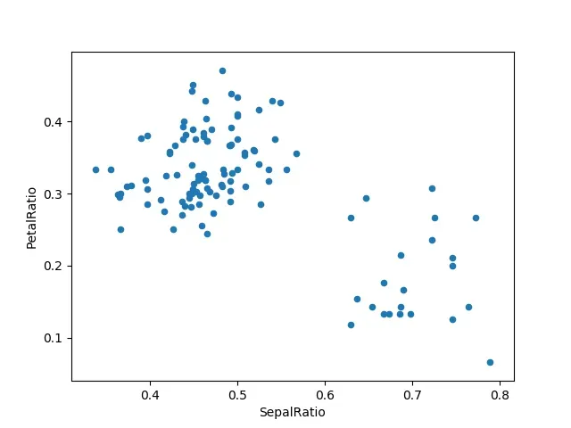
上例用 assign 把函数传递给 DataFrame, 并执行函数运算。这是要注意的是,该 DataFrame 是筛选了花萼长度大于 5 以后的数据。首先执行的是筛选操作,再计算比例。这个例子就是对没有事先筛选 DataFrame 进行的引用。
assign 函数签名就是 **kwargs。键是新字段的列名,值为是插入值(例如,Series 或 NumPy 数组),或把 DataFrame 当做调用参数的函数。返回结果是插入新值的 DataFrame 副本。
0.23.0 版新增。
从 3.6 版开始,Python 可以保存 **kwargs 顺序。这种操作允许依赖赋值,**kwargs 后的表达式,可以引用同一个 assign() 函数里之前创建的列 。(位置函数: 将a的内容移入(解包)到新列表b中。)
In [79]: dfa = pd.DataFrame({"A": [1, 2, 3],
   ....:                     "B": [4, 5, 6]})
   ....:

In [80]: dfa.assign(C=lambda x: x['A'] + x['B'],
   ....:            D=lambda x: x['A'] + x['C'])
   ....:
Out[80]:
   A  B  C   D
0  1  4  5   6
1  2  5  7   9
2 3 6 9 12第二个表达式里,x['C'] 引用刚创建的列,与 dfa['A'] + dfa['B'] 等效。
要兼容所有 Python 版本,可以把 assign 操作分为两部分。
In [81]: dependent = pd.DataFrame({"A": [1, 1, 1]})

In [82]: (dependent.assign(A=lambda x: x['A'] + 1)
   ....:           .assign(B=lambda x: x['A'] + 2))
   ....:
Out[82]:
   A  B
0  2  4
1  2  4
2  2  4
索引 / 选择
索引基础用法如下:
| 操作 | 句法 | 结果 |
|---|---|---|
| 选择列 | df[col] | Series |
| 用标签选择行 (行名称) | df.loc[label] | Series |
| 用整数位置选择行 (行号) | df.iloc[loc] | Series |
| 行切片 | df[5:10] | DataFrame |
| 用布尔向量选择行 | df[bool_vec] | DataFrame |
选择行返回 Series,索引是 DataFrame 的列:
In [83]: df.loc['b']
Out[83]:
one              2
bar              2
flag         False
foo            bar
one_trunc        2
Name: b, dtype: object

In [84]: df.iloc[2]
Out[84]:
one             3
bar             3
flag         True
foo           bar
one_trunc     NaN
Name: c, dtype: object高级索引、切片技巧,请参阅索引.
数据对齐和运算
DataFrame 对象可以自动对齐 ** 列与索引(行标签)** 的数据。与上文一样,生成的结果是列和行标签的并集。
In [85]: df = pd.DataFrame(np.random.randn(10, 4), columns=['A', 'B', 'C', 'D'])

In [86]: df2 = pd.DataFrame(np.random.randn(7, 3), columns=['A', 'B', 'C'])

In [87]: df + df2
Out[87]:
          A         B         C   D
0  0.045691 -0.014138  1.380871 NaN
1 -0.955398 -1.501007  0.037181 NaN
2 -0.662690  1.534833 -0.859691 NaN
3 -2.452949  1.237274 -0.133712 NaN
4  1.414490  1.951676 -2.320422 NaN
5 -0.494922 -1.649727 -1.084601 NaN
6 -1.047551 -0.748572 -0.805479 NaN
7       NaN       NaN       NaN NaN
8       NaN       NaN       NaN NaN
9       NaN       NaN       NaN NaN
DataFrame 和 Series 之间执行操作时,默认操作是在 DataFrame 的列上对齐 Series 的索引,按行执行广播操作。例如:
In [88]: df - df.iloc[0]
Out[88]:
          A         B         C         D
0  0.000000  0.000000  0.000000  0.000000
1 -1.359261 -0.248717 -0.453372 -1.754659
2  0.253128  0.829678  0.010026 -1.991234
3 -1.311128  0.054325 -1.724913 -1.620544
4  0.573025  1.500742 -0.676070  1.367331
5 -1.741248  0.781993 -1.241620 -2.053136
6 -1.240774 -0.869551 -0.153282  0.000430
7 -0.743894  0.411013 -0.929563 -0.282386
8 -1.194921  1.320690  0.238224 -1.482644
9  2.293786  1.856228  0.773289 -1.446531
时间序列是特例,DataFrame 索引包含日期时,按列广播:
In [89]: index = pd.date_range('1/1/2000', periods=8)

In [90]: df = pd.DataFrame(np.random.randn(8, 3), index=index, columns=list('ABC'))

In [91]: df
Out[91]:
                   A         B         C
2000-01-01 -1.226825  0.769804 -1.281247
2000-01-02 -0.727707 -0.121306 -0.097883
2000-01-03  0.695775  0.341734  0.959726
2000-01-04 -1.110336 -0.619976  0.149748
2000-01-05 -0.732339  0.687738  0.176444
2000-01-06  0.403310 -0.154951  0.301624
2000-01-07 -2.179861 -1.369849 -0.954208
2000-01-08  1.462696 -1.743161 -0.826591

In [92]: type(df['A'])
Out[92]: Pandas.core.series.Series

In [93]: df - df['A']
Out[93]:
            2000-01-01 00:00:00  2000-01-02 00:00:00  2000-01-03 00:00:00  2000-01-04 00:00:00  ...  2000-01-08 00:00:00   A   B   C
2000-01-01                  NaN                  NaN                  NaN                  NaN  ...                  NaN NaN NaN NaN
2000-01-02                  NaN                  NaN                  NaN                  NaN  ...                  NaN NaN NaN NaN
2000-01-03                  NaN                  NaN                  NaN                  NaN  ...                  NaN NaN NaN NaN
2000-01-04                  NaN                  NaN                  NaN                  NaN  ...                  NaN NaN NaN NaN
2000-01-05                  NaN                  NaN                  NaN                  NaN  ...                  NaN NaN NaN NaN
2000-01-06                  NaN                  NaN                  NaN                  NaN  ...                  NaN NaN NaN NaN
2000-01-07                  NaN                  NaN                  NaN                  NaN  ...                  NaN NaN NaN NaN
2000-01-08                  NaN                  NaN                  NaN                  NaN  ...                  NaN NaN NaN NaN

[8 rows x 11 columns]
警告
df - df['A']已弃用,后期版本中会删除。实现此操作的首选方法是:
df.sub(df['A'], axis=0)
有关匹配和广播操作的显式控制,请参阅二进制操作。
标量操作与其它数据结构一样:
In [94]: df * 5 + 2
Out[94]:
                   A         B         C
2000-01-01 -4.134126  5.849018 -4.406237
2000-01-02 -1.638535  1.393469  1.510587
2000-01-03  5.478873  3.708672  6.798628
2000-01-04 -3.551681 -1.099880  2.748742
2000-01-05 -1.661697  5.438692  2.882222
2000-01-06  4.016548  1.225246  3.508122
2000-01-07 -8.899303 -4.849247 -2.771039
2000-01-08  9.313480 -6.715805 -2.132955

In [95]: 1 / df
Out[95]:
                   A         B          C
2000-01-01 -0.815112  1.299033  -0.780489
2000-01-02 -1.374179 -8.243600 -10.216313
2000-01-03  1.437247  2.926250   1.041965
2000-01-04 -0.900628 -1.612966   6.677871
2000-01-05 -1.365487  1.454041   5.667510
2000-01-06  2.479485 -6.453662   3.315381
2000-01-07 -0.458745 -0.730007  -1.047990
2000-01-08  0.683669 -0.573671  -1.209788

In [96]: df ** 4
Out[96]:
                    A         B         C
2000-01-01   2.265327  0.351172  2.694833
2000-01-02   0.280431  0.000217  0.000092
2000-01-03   0.234355  0.013638  0.848376
2000-01-04   1.519910  0.147740  0.000503
2000-01-05   0.287640  0.223714  0.000969
2000-01-06   0.026458  0.000576  0.008277
2000-01-07  22.579530  3.521204  0.829033
2000-01-08   4.577374  9.233151  0.466834
支持布尔运算符:
In [97]: df1 = pd.DataFrame({'a': [1, 0, 1], 'b': [0, 1, 1]}, dtype=bool)

In [98]: df2 = pd.DataFrame({'a': [0, 1, 1], 'b': [1, 1, 0]}, dtype=bool)

In [99]: df1 & df2
Out[99]:
       a      b
0  False  False
1  False   True
2   True  False

In [100]: df1 | df2
Out[100]:
      a     b
0  True  True
1  True  True
2  True  True

In [101]: df1 ^ df2
Out[101]:
       a      b
0   True   True
1   True  False
2  False   True

In [102]: -df1
Out[102]:
       a      b
0  False   True
1   True  False
2  False  False
转置
类似于多维数组,T 属性(即 transpose 函数)可以转置 DataFrame:
# only show the first 5 rows
In [103]: df[:5].T
Out[103]:
   2000-01-01  2000-01-02  2000-01-03  2000-01-04  2000-01-05
A   -1.226825   -0.727707    0.695775   -1.110336   -0.732339
B    0.769804   -0.121306    0.341734   -0.619976    0.687738
C   -1.281247   -0.097883    0.959726    0.149748    0.176444
DataFrame 应用 NumPy 函数
Series 与 DataFrame 可使用 log、exp、sqrt 等多种元素级 NumPy 通用函数(ufunc) ,假设 DataFrame 的数据都是数字:
In [104]: np.exp(df)
Out[104]:
                   A         B         C
2000-01-01  0.293222  2.159342  0.277691
2000-01-02  0.483015  0.885763  0.906755
2000-01-03  2.005262  1.407386  2.610980
2000-01-04  0.329448  0.537957  1.161542
2000-01-05  0.480783  1.989212  1.192968
2000-01-06  1.496770  0.856457  1.352053
2000-01-07  0.113057  0.254145  0.385117
2000-01-08  4.317584  0.174966  0.437538

In [105]: np.asarray(df)
Out[105]:
array([[-1.2268,  0.7698, -1.2812],
       [-0.7277, -0.1213, -0.0979],
       [ 0.6958,  0.3417,  0.9597],
       [-1.1103, -0.62  ,  0.1497],
       [-0.7323,  0.6877,  0.1764],
       [ 0.4033, -0.155 ,  0.3016],
       [-2.1799, -1.3698, -0.9542],
       [ 1.4627, -1.7432, -0.8266]])
DataFrame 不是多维数组的替代品,它的索引语义和数据模型与多维数组都不同。
Series 应用 __array_ufunc__,支持 NumPy 通用函数 。
通用函数应用于 Series 的底层数组。
In [106]: ser = pd.Series([1, 2, 3, 4])

In [107]: np.exp(ser)
Out[107]:
0     2.718282
1     7.389056
2    20.085537
3    54.598150
dtype: float64
0.25.0 版更改: 多个 Series 传递给 ufunc 时,会先进行对齐。
Pandas 可以自动对齐 ufunc 里的多个带标签输入数据。例如,两个标签排序不同的 Series 运算前,会先对齐标签。
In [108]: ser1 = pd.Series([1, 2, 3], index=['a', 'b', 'c'])

In [109]: ser2 = pd.Series([1, 3, 5], index=['b', 'a', 'c'])

In [110]: ser1
Out[110]:
a    1
b    2
c    3
dtype: int64

In [111]: ser2
Out[111]:
b    1
a    3
c    5
dtype: int64

In [112]: np.remainder(ser1, ser2)
Out[112]:
a    1
b    0
c    3
dtype: int64
一般来说,Pandas 提取两个索引的并集,不重叠的值用缺失值填充。
In [113]: ser3 = pd.Series([2, 4, 6], index=['b', 'c', 'd'])

In [114]: ser3
Out[114]:
b    2
c    4
d    6
dtype: int64

In [115]: np.remainder(ser1, ser3)
Out[115]:
a    NaN
b    0.0
c    3.0
d    NaN
dtype: float64
# np.remainder(ser1, ser3) 返回除法的元素余数。
对 Series 和 Index 应用二进制 ufunc 时,优先执行 Series,并返回的结果也是 Series 。
In [116]: ser = pd.Series([1, 2, 3])

In [117]: idx = pd.Index([4, 5, 6])

In [118]: np.maximum(ser, idx)
Out[118]:
0    4
1    5
2    6
dtype: int64
NumPy 通用函数可以安全地应用于非多维数组支持的 Series ,例如,SparseArray (参见稀疏计算 )。如有可能,应用 ufunc 而不把基础数据转换为多维数组。
控制台显示
控制台显示大型 DataFrame 时,会根据空间调整显示大小。info() 函数可以查看 DataFrame 的信息摘要。下列代码读取 R 语言 plyr 包里的棒球数据集 CSV 文件):
In [119]: baseball = pd.read_csv('data/baseball.csv')

In [120]: print(baseball)
       id     player  year  stint team  lg   g   ab   r    h  X2b  X3b  hr   rbi   sb   cs  bb    so  ibb  hbp   sh   sf  gidp
0   88641  womacto01  2006      2  CHN  NL  19   50   6   14    1    0   1   2.0  1.0  1.0   4   4.0  0.0  0.0  3.0  0.0   0.0
1   88643  schilcu01  2006      1  BOS  AL  31    2   0    1    0    0   0   0.0  0.0  0.0   0   1.0  0.0  0.0  0.0  0.0   0.0
..    ...        ...   ...    ...  ...  ..  ..  ...  ..  ...  ...  ...  ..   ...  ...  ...  ..   ...  ...  ...  ...  ...   ...
98  89533   aloumo01  2007      1  NYN  NL  87  328  51  112   19    1  13  49.0  3.0  0.0  27  30.0  5.0  2.0  0.0  3.0  13.0
99  89534  alomasa02  2007      1  NYN  NL   8   22   1    3    1    0   0   0.0  0.0  0.0   0   3.0  0.0  0.0  0.0  0.0   0.0

[100 rows x 23 columns]

In [121]: baseball.info()
<class 'Pandas.core.frame.DataFrame'>
RangeIndex: 100 entries, 0 to 99
Data columns (total 23 columns):
id        100 non-null int64
player    100 non-null object
year      100 non-null int64
stint     100 non-null int64
team      100 non-null object
lg        100 non-null object
g         100 non-null int64
ab        100 non-null int64
r         100 non-null int64
h         100 non-null int64
X2b       100 non-null int64
X3b       100 non-null int64
hr        100 non-null int64
rbi       100 non-null float64
sb        100 non-null float64
cs        100 non-null float64
bb        100 non-null int64
so        100 non-null float64
ibb       100 non-null float64
hbp       100 non-null float64
sh        100 non-null float64
sf        100 non-null float64
gidp      100 non-null float64
dtypes: float64(9), int64(11), object(3)
memory usage: 18.1+ KB
尽管 to_string 有时不匹配控制台的宽度,但还是可以用 to_string 以表格形式返回 DataFrame 的字符串表示形式:
In [122]: print(baseball.iloc[-20:, :12].to_string())
       id     player  year  stint team  lg    g   ab   r    h  X2b  X3b
80  89474  finlest01  2007      1  COL  NL   43   94   9   17    3    0
81  89480  embreal01  2007      1  OAK  AL    4    0   0    0    0    0
82  89481  edmonji01  2007      1  SLN  NL  117  365  39   92   15    2
83  89482  easleda01  2007      1  NYN  NL   76  193  24   54    6    0
84  89489  delgaca01  2007      1  NYN  NL  139  538  71  139   30    0
85  89493  cormirh01  2007      1  CIN  NL    6    0   0    0    0    0
86  89494  coninje01  2007      2  NYN  NL   21   41   2    8    2    0
87  89495  coninje01  2007      1  CIN  NL   80  215  23   57   11    1
88  89497  clemero02  2007      1  NYA  AL    2    2   0    1    0    0
89  89498  claytro01  2007      2  BOS  AL    8    6   1    0    0    0
90  89499  claytro01  2007      1  TOR  AL   69  189  23   48   14    0
91  89501  cirilje01  2007      2  ARI  NL   28   40   6    8    4    0
92  89502  cirilje01  2007      1  MIN  AL   50  153  18   40    9    2
93  89521  bondsba01  2007      1  SFN  NL  126  340  75   94   14    0
94  89523  biggicr01  2007      1  HOU  NL  141  517  68  130   31    3
95  89525  benitar01  2007      2  FLO  NL   34    0   0    0    0    0
96  89526  benitar01  2007      1  SFN  NL   19    0   0    0    0    0
97  89530  ausmubr01  2007      1  HOU  NL  117  349  38   82   16    3
98  89533   aloumo01  2007      1  NYN  NL   87  328  51  112   19    1
99  89534  alomasa02  2007      1  NYN  NL    8   22   1    3    1    0
默认情况下,过宽的 DataFrame 会跨多行输出:
In [123]: pd.DataFrame(np.random.randn(3, 12))
Out[123]:
          0         1         2         3         4         5         6         7         8         9        10        11
0 -0.345352  1.314232  0.690579  0.995761  2.396780  0.014871  3.357427 -0.317441 -1.236269  0.896171 -0.487602 -0.082240
1 -2.182937  0.380396  0.084844  0.432390  1.519970 -0.493662  0.600178  0.274230  0.132885 -0.023688  2.410179  1.450520
2  0.206053 -0.251905 -2.213588  1.063327  1.266143  0.299368 -0.863838  0.408204 -1.048089 -0.025747 -0.988387  0.094055
display.width 选项可以更改单行输出的宽度:
In [124]: pd.set_option('display.width', 40)  # 默认值为 80

In [125]: pd.DataFrame(np.random.randn(3, 12))
Out[125]:
          0         1         2         3         4         5         6         7         8         9        10        11
0  1.262731  1.289997  0.082423 -0.055758  0.536580 -0.489682  0.369374 -0.034571 -2.484478 -0.281461  0.030711  0.109121
1  1.126203 -0.977349  1.474071 -0.064034 -1.282782  0.781836 -1.071357  0.441153  2.353925  0.583787  0.221471 -0.744471
2  0.758527  1.729689 -0.964980 -0.845696 -1.340896  1.846883 -1.328865  1.682706 -1.717693  0.888782  0.228440  0.901805
还可以用 display.max_colwidth 调整最大列宽。
In [126]: datafile = {'filename': ['filename_01', 'filename_02'],
   .....:             'path': ["media/user_name/storage/folder_01/filename_01",
   .....:                      "media/user_name/storage/folder_02/filename_02"]}
   .....:

In [127]: pd.set_option('display.max_colwidth', 30)

In [128]: pd.DataFrame(datafile)
Out[128]:
      filename                           path
0  filename_01  media/user_name/storage/fo...
1  filename_02  media/user_name/storage/fo...

In [129]: pd.set_option('display.max_colwidth', 100)

In [130]: pd.DataFrame(datafile)
Out[130]:
      filename                                           path
0  filename_01  media/user_name/storage/folder_01/filename_01
1  filename_02  media/user_name/storage/folder_02/filename_02
expand_frame_repr 选项可以禁用此功能,在一个区块里输出整个表格。
DataFrame 列属性访问和 IPython 代码补全
DataFrame 列标签是有效的 Python 变量名时,可以像属性一样访问该列:
In [131]: df = pd.DataFrame({'foo1': np.random.randn(5),
   .....:                    'foo2': np.random.randn(5)})
   .....:

In [132]: df
Out[132]:
       foo1      foo2
0  1.171216 -0.858447
1  0.520260  0.306996
2 -1.197071 -0.028665
3 -1.066969  0.384316
4 -0.303421  1.574159

In [133]: df.foo1
Out[133]:
0    1.171216
1    0.520260
2   -1.197071
3   -1.066969
4   -0.303421
Name: foo1, dtype: float64
IPython 支持补全功能,按 tab 键可以实现代码补全:
In [134]: df.fo<TAB>  # 此时按 tab 键 会显示下列内容
df.foo1  df.foo2
文章出处登录后可见!