目录
1.Anomaly Detection — Gaussian Distribution
3.Multivariant Gaussian Distribution
5.Stochastic/Mini-batch Grandient Descent
前言
从高斯到完结
最后两周的内容不多。就合在一起写了。
一、进度
第九周、第十周、第十一周(100%)
二、基本内容
1.Anomaly Detection — Gaussian Distribution
在聚类问题的时候,我们有时候会发现有聚类异常的情况。如何把聚类错误的点区分出来,可以用到之前高斯核的思路:将葛店投影到高维空间进行区分。
这里使用了进行高斯分布的方法,在一定ε的取值范围内选择合理的正例和反例。高斯分布的μ和δ需要经过合理选择。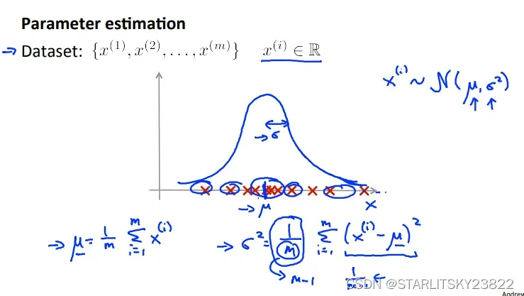
一般来说会出现多维的特征,会有很多很多的Xi。将各个Xi融入进一个高斯分布的方法是将各个Xi的高斯分布的参数进行累乘。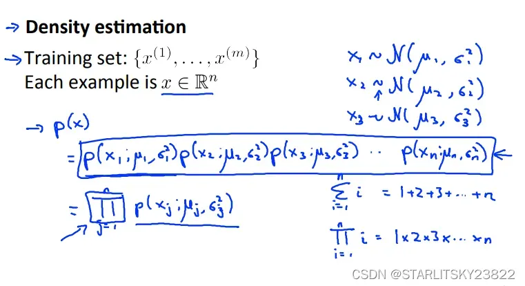
至于如何确定μ和δ,运用高斯分布的定义式即可。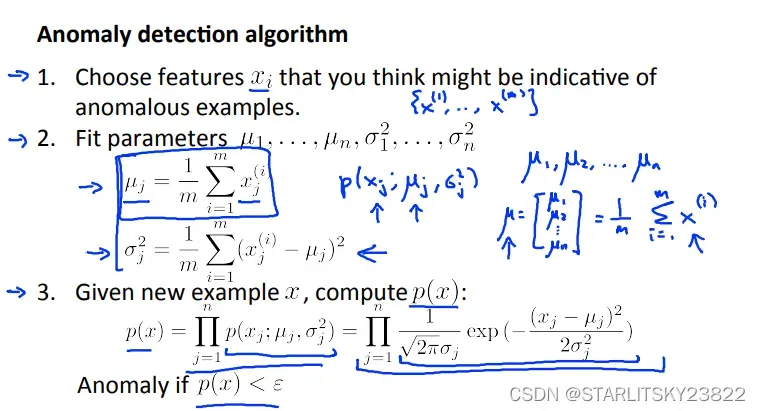
对于评价我们进行选择正反例的ε,我们可以使用之前学过的recall值、precision值或者综合的F1值进行评价。如果算出来的F1评估值在可接受阈值之上,那我们认为ε是合理的。
同时,注意anomaly detection和监督学习的使用区别。简单来说,使用AD的情况就是类似飞机引擎异常检测的例子:有足够多的反例(没有问题的引擎),只有比较少的正例(有问题的引擎)。系统没有办法从足够多的正例中学习到特征(这就是监督学习的拟合部分了)。虽然我觉得有点怪,正反例不是人为规定的吗?
2.Choosing Features
对于非高斯分布的样本,我们可以对其进行合理的数学变换,最终变为高斯分布的形式: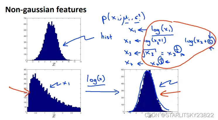
同时,我们可以对特征规定某种运算规则,使得我们想要的特定情况下的某个值会和我们进行检测的数值称高斯分布的函数关系: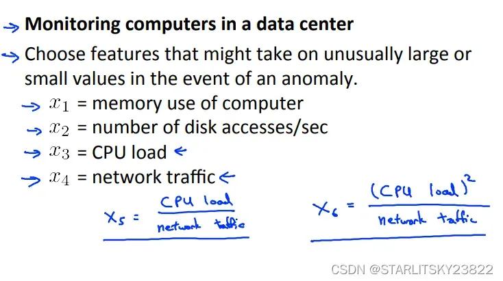
3.Multivariant Gaussian Distribution
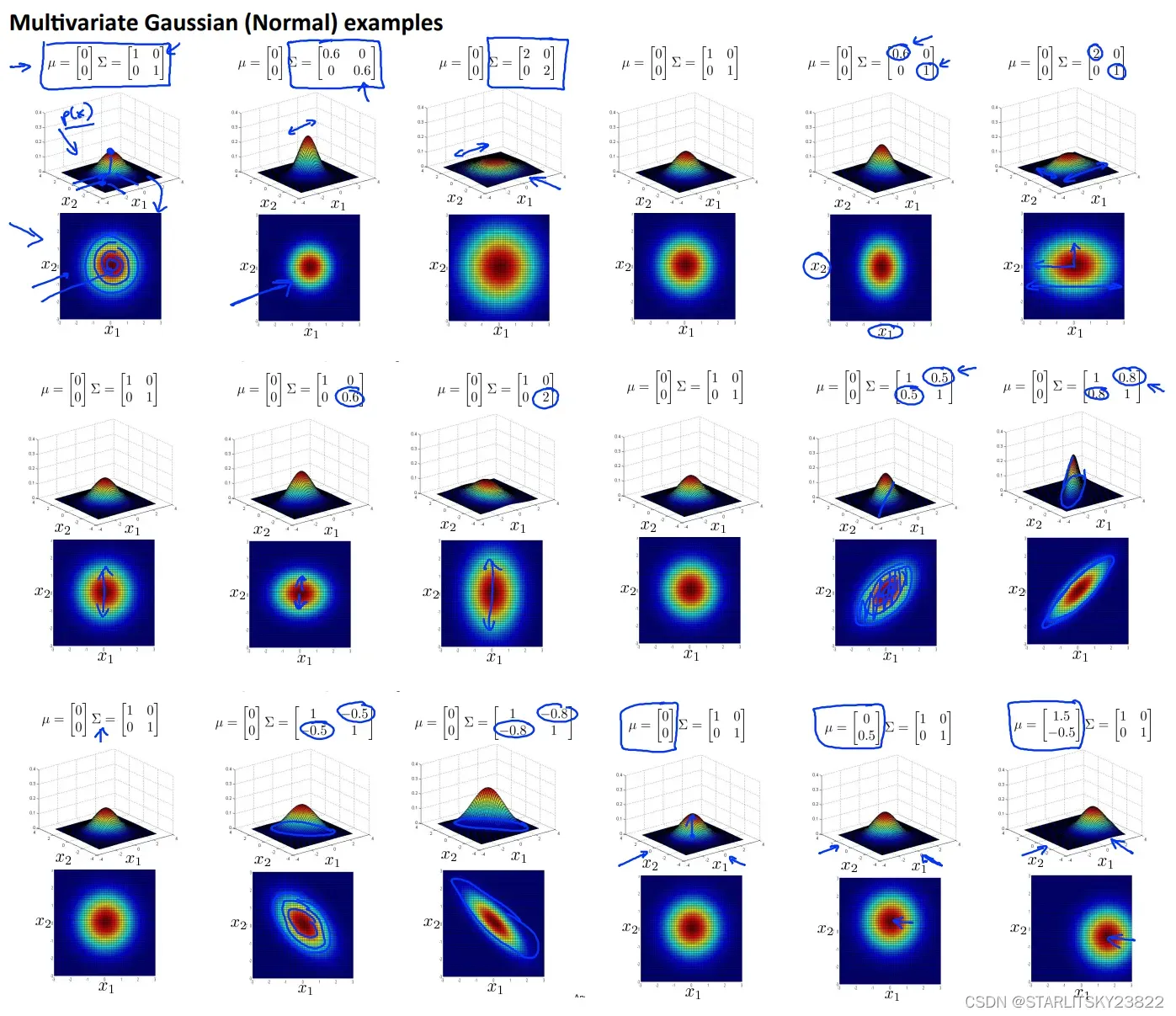
有时候在三维情况下,我们的特征分布是长成高斯分布形状的,但是在具体细节上会有差距,比如分布的高低,范围,还有沿某些特定的角度会有数值的分离。这时候我们要修改高斯分布函数的形式: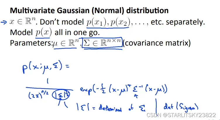
对于用协方差矩阵∑代替δ进行运算,本身的运算过程如下: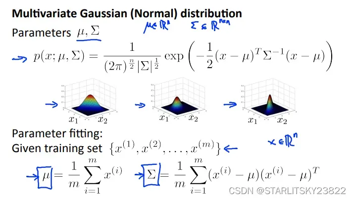 这里可以注意到使用协方差矩阵进行计算和之前我们使用累乘进行计算的方法有区别。最本质的区别就是使用累乘方法是和我们手动选择某些特征联系在一起的(比如CPU^2/内存),而协方差矩阵则自带了特征矩阵的属性。
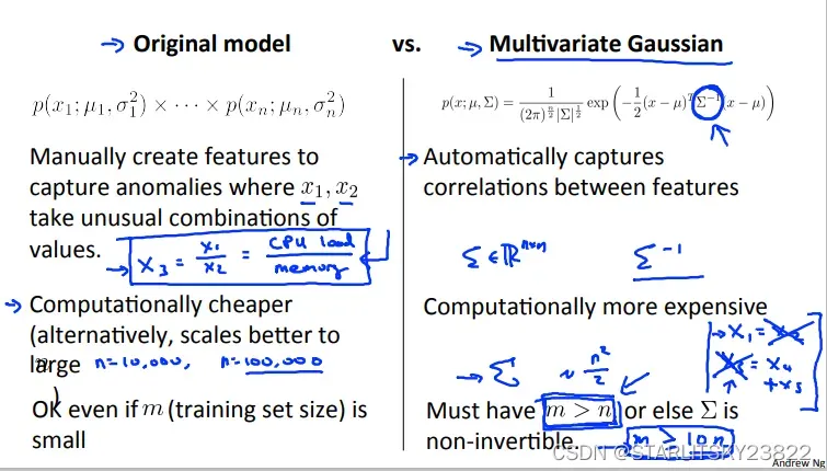
4.Recommander System
推荐系统简单一览。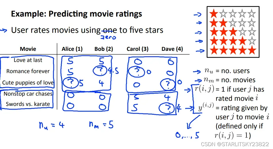
同时引入两个矩阵X和θ,X是电影的属性矩阵,1*n维,比如维数分别对应爱情指数,恐怖指数,悬疑指数等等。θ是观众指数,相对应的,表示该观众对爱情元素,恐怖元素,悬疑元素的感冒程度。下图中的最后一行就是简单的监督学习,来得到最接近该观众的θ。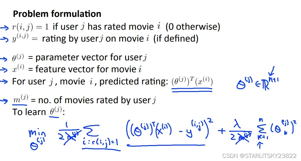
同样的,相反如果我们不知道X但是知道θ,我们也可以根据观众给出的打分结合θ来确定该电影的X属性矩阵。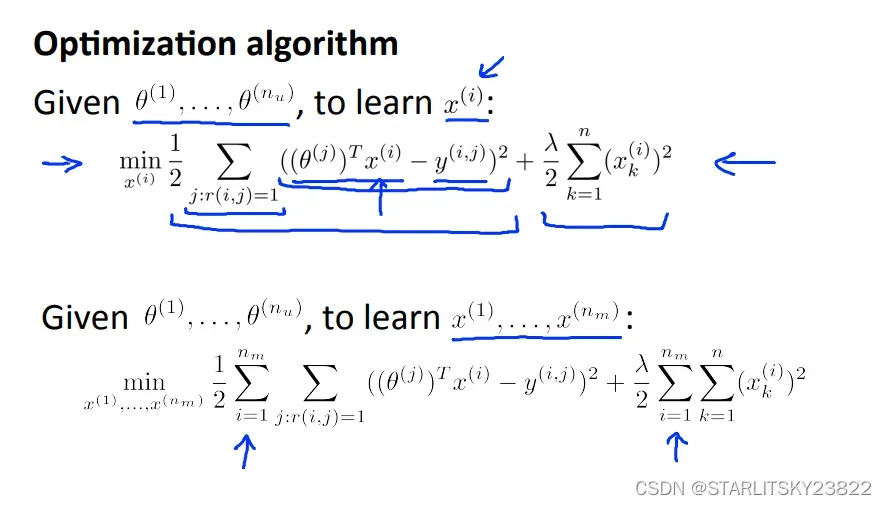
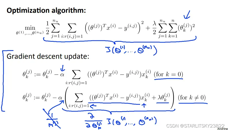
那么这里就有问题了,我们是都知道了θ或者X中的一个,然后去最优化另一个。如果我们两个都不知道,那么我们就要同时minX和θ决定的cost fuction。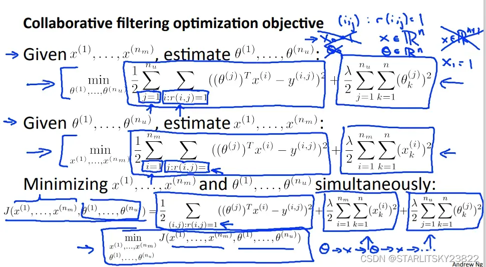
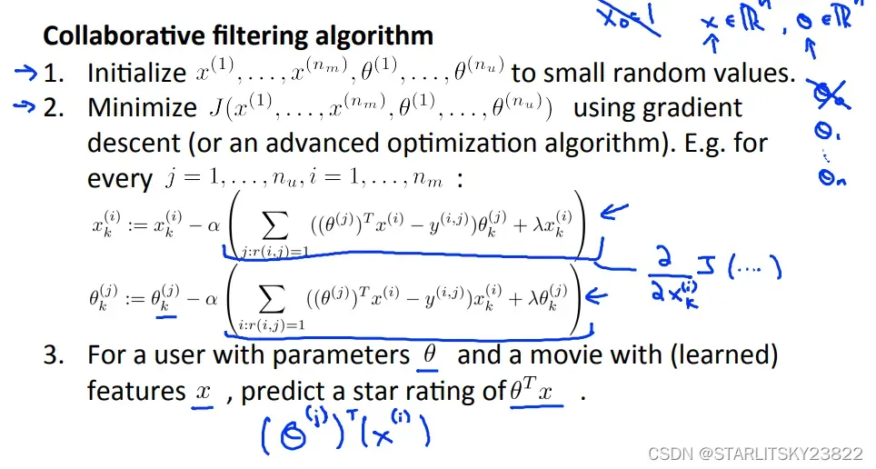
对于有一些电影,观众没有给出评分,我们的做法是将该电影的X值取出,然后找到和这部电影的X值比较接近的电影(||Xi-Xj||²最小的几部电影)。然后将θ和X进行运算。这部分没有展开讲,直接略过。
同时,有时候电影的给分比较两极化。所以我们也可以使用类似Feature Scaling的操作: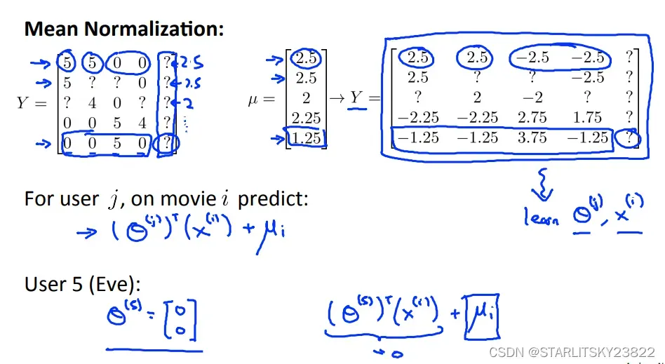
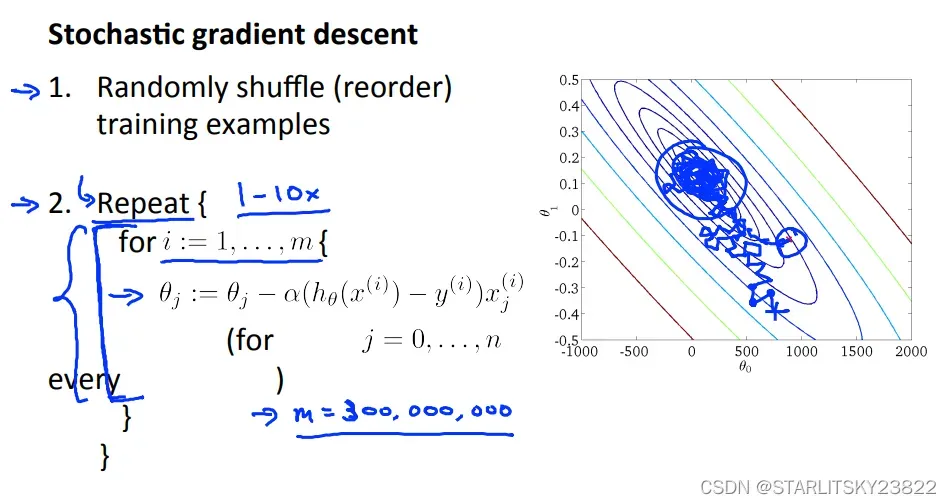
5.Stochastic/Mini-batch Grandient Descent
在之前的梯度下降法中,我们是将所有的值都用于计算Loss以及求偏导,但是在随机梯度下降里面我们每使用一个样本就进行梯度下降。虽然之前的梯度下降保证了向全局最优解靠近,但是开销过大。而随机梯度下降虽然没法保证每次都向着最优解靠近,但是当样本数达到一定程度时,我们可以相信随机梯度下降能够到达我们想要的最优解。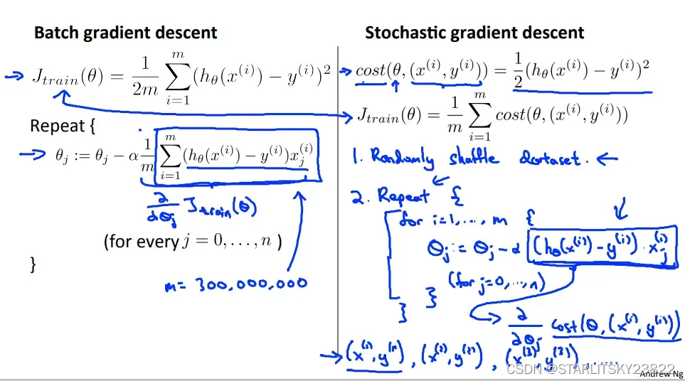
如果研究随机梯度下降的相关曲线,我们会有下图。图一表示不同大小的学习率(和图4区分,这两个学习率都是比较小的且合理的),图二表示样本数量,图三表示你写的算法有问题,吐司表示学习率太大。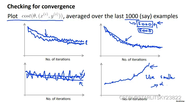
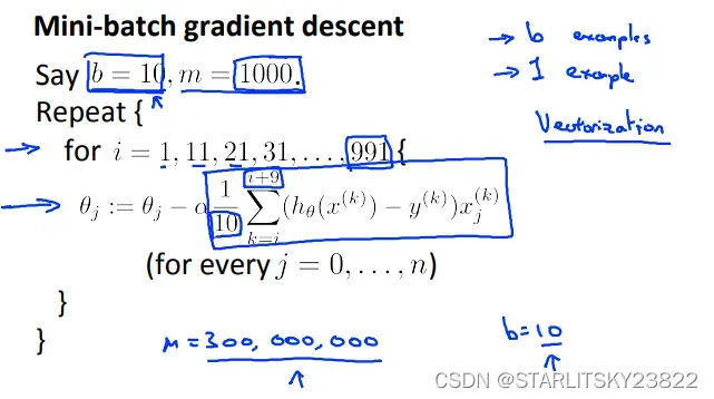
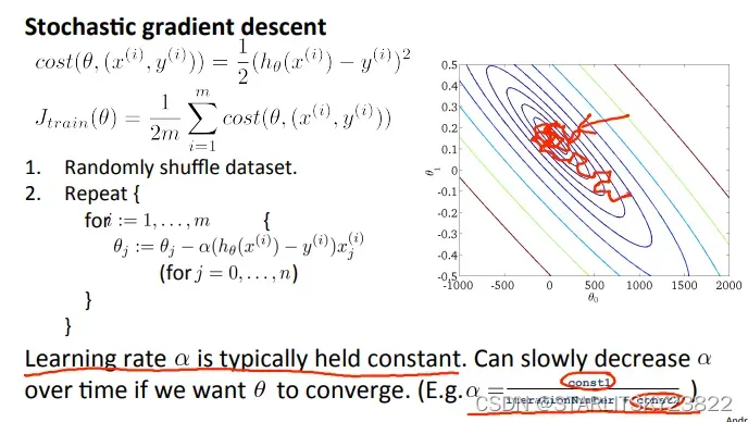 在小规模梯度下降的时候,就是结合了前面的梯度下降和随机梯度下降,选取一部分样本作为梯度下降的Loss和求偏导部分。
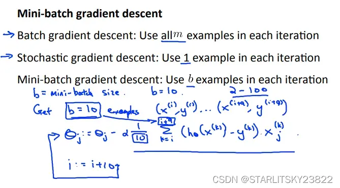
6.Online Learning and Map-reduce and Data Parallelism
首先对于线上学习,以网点为例。假如用户输入的是某些关键字,我们该怎么评价对应的推荐算法的优劣呢?我们选用推荐商品的点击率作为评价标准。点击率来决定算法的实施。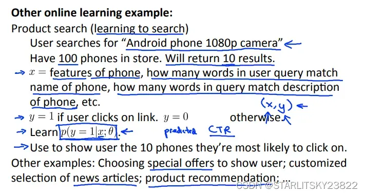
对于Map-reduce,是一个在机器学习领域广泛使用的一个新应用。基本思路就是使用并行系统,将所需计算的工作量平均分给多个计算单元,可以节约计算时间。有时候,单台计算机我们也可以用多核CPU模拟该过程。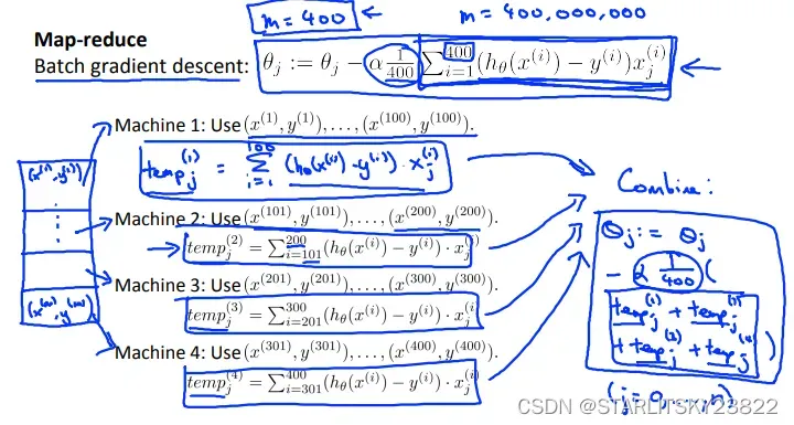
7.Application Example: OCR
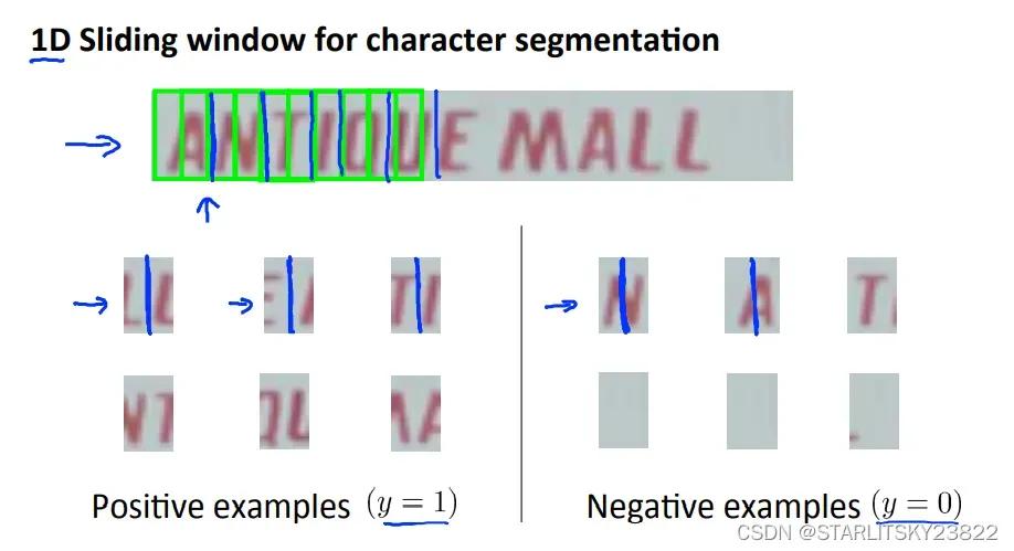
首先有些概念,例如sliding window。
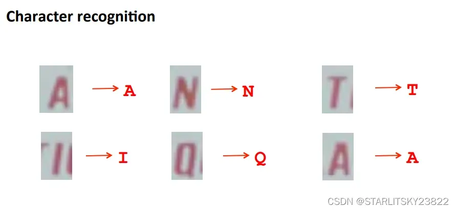
然后详解OCR的过程。首先先对图像进行遍历。遍历的方式是选用特定的图像选择框,然后在特定的图像选择框内判断有无字体。以人行道上的行人检测系统为例,在一整个画面之中,有特定大小的选择框以特定的速率从左至右进行移动,判断出在该选择框内有无具体的行人,应用到OCR问题中,就是判断具体的某个框中有无字母。判断框中物体本身也是一个监督学习的问题。判断完成后,即可形成在特定的选框下被识别出来的字体图像。我们可以采用放大特征点的方法。即在一张黑白区分的图像里,将代表识别出有字的白色区域进行邻域的放大,然后放大特征区域后的黑白色块照片与原图进行叠加,从而保证不会有特征的遗漏。然后,我们对于特定白色区域的文字进行分割。而分割本身又是一类监督学习的问题。将文字进行正确的分割后,形成了文字的叠加为词语。有时候识别文字会出现错误,比如识别出了一个单词c1ever,那我们可以人为将识别错误的单词进行修正。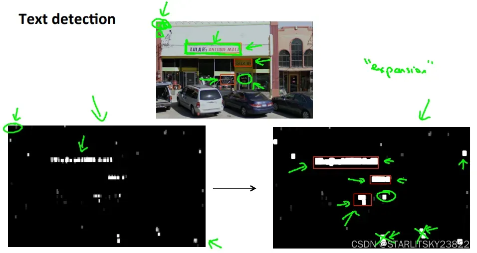
同时我们为了训练我们的算法,我们可以从有限的例子中改编例子将其变为新的训练样本。比如对某些样本进行一些修改。例如在声音识别里,加入背景噪音即可获得新的样本。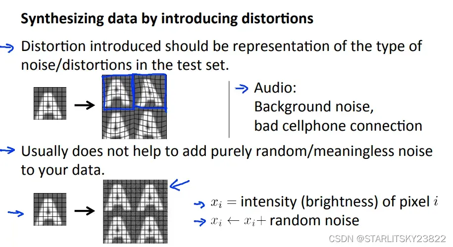
然后讨论pipeline,它能有效提升我们的优化效率。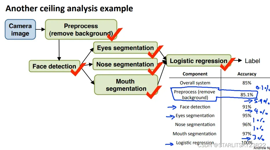
在上述例子中,我们采取的办法就是对于每一个模块的前驱模块,给出客观正确的前驱模块,然后评价后续模块的精确度提升。对于那些精度提升特别大的模块,可以认为提升空间很大。其实这一步就是评价哪些模块值得我们花时间去改善。另外,Andrew式嘲讽:“There was a computer vision application where there’s a team of two engineers that literally spent about a year and a half working on better background removal, actually worked but really complicated algorithms and ended up publishing one research paper. But after all that work they found that it just did not make huge difference to the overall performance of the actual application they were working on and if only someone were to do ceiling analysis before hand maybe they could have realized. And one of them said to me afterward. If only you’ve did this sort of analysis like this maybe they could have realized before their 18 months of work. ”
8.作业
时间有点久远,只记得做下来没什么问题。
function [mu sigma2] = estimateGaussian(X)
%ESTIMATEGAUSSIAN This function estimates the parameters of a
%Gaussian distribution using the data in X
%   [mu sigma2] = estimateGaussian(X),
%   The input X is the dataset with each n-dimensional data point in one row
%   The output is an n-dimensional vector mu, the mean of the data set
%   and the variances sigma^2, an n x 1 vector
%

% Useful variables
[m, n] = size(X);

% You should return these values correctly
mu = zeros(n, 1);
sigma2 = zeros(n, 1);

% ====================== YOUR CODE HERE ======================
% Instructions: Compute the mean of the data and the variances
%               In particular, mu(i) should contain the mean of
%               the data for the i-th feature and sigma2(i)
%               should contain variance of the i-th feature.
%

for i = 1:n
  mu(i) = (1/m)*sum(X(:,i));
end
for i = 1:n
  sume = 0;
  for j = 1:m
    sume = sume + (X(j,i)-mu(i))^2;
  endfor
  sigma2(i) = sume/m;
end
% =============================================================


end
function [bestEpsilon bestF1] = selectThreshold(yval, pval)
%SELECTTHRESHOLD Find the best threshold (epsilon) to use for selecting
%outliers
% [bestEpsilon bestF1] = SELECTTHRESHOLD(yval, pval) finds the best
% threshold to use for selecting outliers based on the results from a
% validation set (pval) and the ground truth (yval).
%
bestEpsilon = 0;
bestF1 = 0;
F1 = 0;
stepsize = (max(pval) - min(pval)) / 1000;
for epsilon = min(pval):stepsize:max(pval)
% ====================== YOUR CODE HERE ======================
% Instructions: Compute the F1 score of choosing epsilon as the
% threshold and place the value in F1. The code at the
% end of the loop will compare the F1 score for this
% choice of epsilon and set it to be the best epsilon if
% it is better than the current choice of epsilon.
%
% Note: You can use predictions = (pval < epsilon) to get a binary vector
% of 0's and 1's of the outlier predictions
predictions = (pval < epsilon);
tp = 0;
fp = 0;
fn = 0;
for i = 1 : sizeof(predictions)
if(predictions(i)==1 && yval(i)==1)
tp = tp+1;
elseif(predictions(i)==1 && yval(i)==0)
fp = fp+1;
elseif(predictions(i)==0 && yval(i)==1)
fn = fn+1;
endif
endfor
prec = tp/(tp + fp);
rec = tp/(tp + fn);
F1 = 2*prec*rec/(prec + rec);
% =============================================================
if F1 > bestF1
bestF1 = F1;
bestEpsilon = epsilon;
end
end
endfunction [J, grad] = cofiCostFunc(params, Y, R, num_users, num_movies, ...
num_features, lambda)
%COFICOSTFUNC Collaborative filtering cost function
% [J, grad] = COFICOSTFUNC(params, Y, R, num_users, num_movies, ...
% num_features, lambda) returns the cost and gradient for the
% collaborative filtering problem.
%
% Unfold the U and W matrices from params
X = reshape(params(1:num_movies*num_features), num_movies, num_features);
Theta = reshape(params(num_movies*num_features+1:end), ...
num_users, num_features);
% You need to return the following values correctly
J = 0;
X_grad = zeros(size(X));
Theta_grad = zeros(size(Theta));
% ====================== YOUR CODE HERE ======================
% Instructions: Compute the cost function and gradient for collaborative
% filtering. Concretely, you should first implement the cost
% function (without regularization) and make sure it is
% matches our costs. After that, you should implement the
% gradient and use the checkCostFunction routine to check
% that the gradient is correct. Finally, you should implement
% regularization.
%
% Notes: X - num_movies x num_features matrix of movie features
% Theta - num_users x num_features matrix of user features
% Y - num_movies x num_users matrix of user ratings of movies
% R - num_movies x num_users matrix, where R(i, j) = 1 if the
% i-th movie was rated by the j-th user
%
% You should set the following variables correctly:
%
% X_grad - num_movies x num_features matrix, containing the
% partial derivatives w.r.t. to each element of X
% Theta_grad - num_users x num_features matrix, containing the
% partial derivatives w.r.t. to each element of Theta
%
J = (1/2)*sum(sum(((X*Theta'.*R)-Y).^2));
X_grad = ((X*Theta'.*R)-Y)*Theta;
Theta_grad = ((X*Theta'.*R)-Y)'*X;
J = J + (lambda/2)*sum(sum(Theta.^2)) + (lambda/2)*sum(sum(X.^2));
X_grad = X_grad + lambda * X;
Theta_grad = Theta_grad + lambda * Theta;
% =============================================================
grad = [X_grad(:); Theta_grad(:)];
end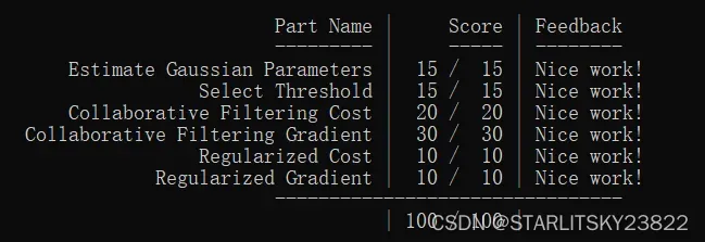
总结
这次的总结没有什么意思,就放到下一篇的课程总结里来写吧。
文章出处登录后可见!