paper：Boundary loss for highly unbalanced segmentation

Introduction

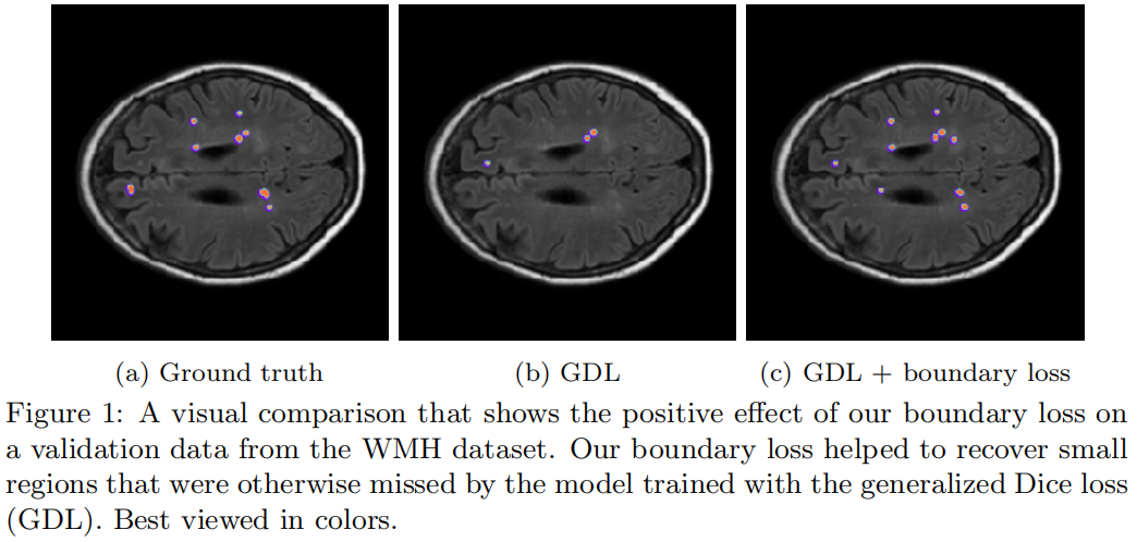
在医学图像分割中任务中通常存在严重的类别不平衡问题，目标前景区域的大小常常比背景区域小几个数量级，比如下图中前景区域比背景区域小500倍以上。

分割通常采用的交叉熵损失函数，在高度不平衡的问题上存在着众所周知的缺点即它假设所有样本和类别的重要性相同，这通常会导致训练的不稳定，并导致决策边界偏向于数量多的类别。对于类别不平衡问题，一种常见的策略是对数目多的类别进行降采样来重新平衡类别的先验分布，但是这种策略限制了训练图像的使用。另一种策略是加权，即对数量少的类别赋予更大的权重，对数量多的类别赋予更小的权重，虽然这种方法对一些不平衡的问题是有效的，但处理极度不平衡的数据时还是有困难。在少数几个像素上计算的交叉熵梯度通常包含了噪声，赋予少数类别更大的权重进一步加大了噪声从而导致训练的不稳定。

分割中另一种常见的损失函数dice loss，在不平衡的医学图像分割问题中通常比ce loss的效果好。但遇到非常小的区域时可能会遇到困难，错误分类的像素可能会导致loss的剧烈降低，从而导致优化的不稳定。此外，dice loss对应精度和召回的调和平均，当true positive不变时，false postive和false negative重要性相同，因此dice loss主要适用于这两种类型的误差数量差不多的情况。

Contributions

CE loss和Dice loss分别是基于分布和基于区域的损失函数，本文提出了一种基于边界的损失函数，它在轮廓空间而不是区域空间上采用距离度量的形式。边界损失计算的不是区域上积分，而是区域之间边界上积分，因此可以缓解高度不平衡分割问题中区域损失的相关问题。

但是怎么根据CNN的regional softmax输出来表示对应的boundary points是个很大的挑战，本文受到用离散基于图的优化方法来计算曲线演化梯度流的启发，采用积分方法来计算边界的变化，避免了轮廓点上的局部微分计算，最终的boundary loss是网络输出区域softmax概率的线性函数和，因此可以和现有的区域损失结合使用。

Formulation

 \(I:\Omega \subset \mathbb{R}^{2,3}\rightarrow \mathbb{R}\) 表示空间域 \(\Omega\) 中的一张图片，\(g:\Omega \rightarrow \begin{Bmatrix}
0,1
\end{Bmatrix}\) 是该图片的ground truth分割二值图，如果像素 \(p\) 属于目标区域 \(G\subset \Omega\) （前景区域），\(g(p)=1\)，否则为0，即 \(p\in\Omega\setminus G\)（背景区域）。\(s_{\theta}:\Omega\rightarrow [0,1]\) 表示分割网络的softmax概率输出，\(S_{\theta}\subset\Omega\) 表示模型输出的对应前景区域即 \(S_{\theta}=\begin{Bmatrix}
p\in\Omega|s_{\theta}(p)\geqslant \delta 
\end{Bmatrix}\)，其中 \(\delta\) 是提前设定的阈值。

我们的目的是构建一个边界损失函数 \(Dist(\partial G,\partial S_{\theta })\)，它采用 \(\Omega\) 中区域边界空间中距离度量的形式，其中 \(\partial G\) 是ground truth区域 \(G\) 的边界的一种表示（比如边界上所有点的集和），\(\partial S_{\theta }\) 是网络输出定义的分割区域的边界。如何将 \(\partial S_{\theta }\) 上的点表示成网络输出区域 \(s_{\theta }\) 的可导函数尚不清楚。考虑下面的形状空间上非对称 \(L_{2}\ distance\) 的表示，它评估的是两个临近边界 \(\partial S\) 和 \(\partial G\) 之间的距离变化

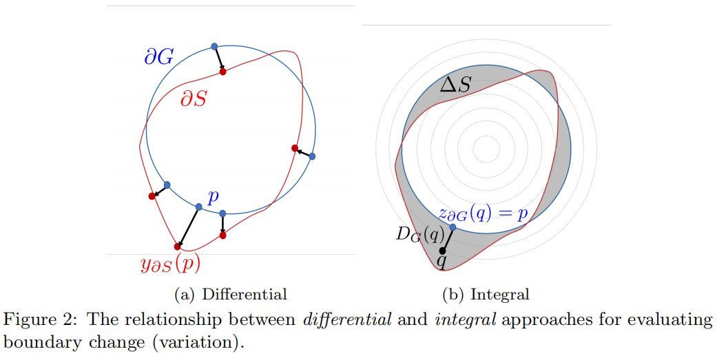
其中 \(p\in\Omega\) 是边界 \(\partial G\) 上的一点，\(y_{\partial S}(p)\) 是边界 \(\partial S\) 上对应的点，即 \(y_{\partial S}(p)\) 是 \(\partial G\) 上点 \(p\) 处的发现与 \(\partial S\) 的交点，如图2(a)所示，\(\left \| \cdot  \right \|\) 表示 \(L_{2}\) 范数。和其它直接调用轮廓 \(\partial S\)上点的轮廓军距离一样，对于 \(\partial S=\partial S_{\theta}\) 式(2)不能直接作为loss函数使用。但是很容易证明式(2)中的微分边界变化可以用积分方法来近似，这就避免了涉及轮廓上点的微分计算，并用区域积分来表示边界变化，如下

其中 \(\bigtriangleup S\) 表示两个轮廓之间的区域，\(D_{G}:\Omega\rightarrow \mathbb{R}^{+}\) 是一个相对于边界 \(\partial G\) 的distance map，即 \(D_{G}(q)\) 表示任意点 \(q\in\Omega\) 与轮廓 \(\partial G\) 上最近点 \(z_{\partial G}(q)\) 之间的距离：\(D_{G}(q)=\left \| q-z_{\partial G}(q) \right \|\)，如图2(b)所示。

为了证明这种近似，沿连接 \(\partial G\) 上的一点 \(p\) 与 \(y_{\partial S}(p)\) 之间的法线对距离图 \(2D_{G}(q)\) 进行积分通过如下的转换可得 \(\left \| y_{\partial S(p)}-p \right \|^{2}\)

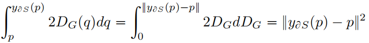
由式(3)进一步得到下式

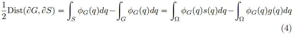
其中 \(s:\Omega\rightarrow \left \{ 0,1 \right \}\) 是区域 \(S\) 的二元指示函数：\(s(q)=1\ if\ q\in S\) 属于目标否则为0。\(\phi _{G}:\Omega\rightarrow \mathbb{R}\) 是边界 \(\partial G\) 的水平集表示：\(\phi _{G}(q)=-D_{G}(q)\ if\ q\in G\) 否则 \(\phi _{G}(q)=D_{G}(q)\)。对于 \(S=S_{\theta}\)，即用网络的softmax输出 \(s_{\theta}(q)\) 替换式(4)中的 \(s(q)\)，我们就得到了如下所示的边界损失

注意我们去掉了式(4)中的最后一项，因为它不包含模型参数。水平集函数 \(\phi_{G}\) 是直接根据gt区域 \(G\) 提前计算得到的。边界损失可以与常用的基于区域的损失函数结合起来用于 \(N\) 类的分割问题

其中 \(\alpha \in\mathbb{R}\) 是平衡两个损失的权重参数。

在式(5)中，每个点 \(q\) 的softmax输出通过距离函数进行加权，在基于区域的损失函数中，这种到边界距离的信息被忽略了，区域内每个点不管到边界距离大小都都按同样的权重进行处理。

在作者提出的边界损失中，当距离函数中所有的负值都保留（模型对即gt区域中所有像素的softmax预测都为1）而所有的正值都舍去（即模型对背景的softmax预测都为0）时，边界损失到达全局最小，即模型的softmax预测正好输出ground truth时边界损失最小，这也验证了边界损失的有效性。

在后续的实验中可以看到，通常要把边界损失和区域损失结合起来使用才能取得好的效果。作者在文中解释的原因没太看懂，贴一下原文

 "As discussed earlier, the global optimum of our boundary loss corresponds to a strictly negative value, with the softmax probabilities yielding a non-empty foreground region. However, an empty foreground, with approximately null values of the softmax probabilities almost everywhere, corresponds to very low gradients. Therefore, this trivial solution is close to a local minimum or a saddle point. This is why we integrate our boundary loss with a regional loss"

Experiments

Comparision of regional losses

在于其它损失函数的对比实验中，\alpha采用rebalance策略，即初始值为0.01，每个epoch后增加0.01。

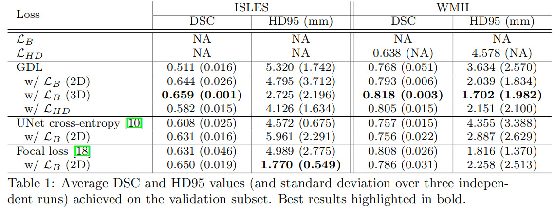
从表中可以看到不管是cross-entropy loss、general dice loss还是focal loss，在于boundary loss结合使用后都获得了一定的精度提升，表明了边界损失的有效性。 

Selection of \(\alpha\)

作者对比了三种不同的方式，一是constant \(\alpha\)，即在整个训练过程中 \(\alpha\) 的值保持不变；二是increase \(\alpha\)，即初始设置为一个大于0但比较小的值，在每个epoch结束后逐渐增加 \(\alpha\)值，但区域损失的权重保持不变，直到训练结束，两种损失的权重一样大；三是rebalance \(\alpha\)，即按 \((1-\alpha)L_{R}+\alpha L_{B}\) 的方式组合两种损失，每个epoch后增加 \(\alpha\) 的值，随着训练的进行边界损失的权重越来越大，而区域损失的权重越来越小。实验结果如下

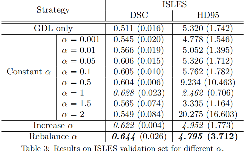
可以看出，Rebalance的策略获得了最优结果，因此在于其它区域损失的结果对比实验中，也全部使用了该策略。

Implementation

其中data是ground truth，这里只考虑二分类的情况，即前景和背景。logits是softmax后的输出，这里为了方便相当于通过argmax或是阈值的方式将模型输出中的每个像素划分到对应类别了，实际上这里的值应该是softmax的输出，介于[0, 1]之间。其中计算distance map是通过scipy库中的distance_transform_edt函数，关于这个函数的介绍可参考 scipy.ndimage.distance_transform_edt 和 cv2.distanceTransform用法

import torch
import numpy as np
from torch import einsum
from torch import Tensor
from scipy.ndimage import distance_transform_edt as distance
from typing import Any, Callable, Iterable, List, Set, Tuple, TypeVar, Union


# switch between representations
def probs2class(probs: Tensor) -> Tensor:
    b, _, w, h = probs.shape  # type: Tuple[int, int, int, int]
    assert simplex(probs)

    res = probs.argmax(dim=1)
    assert res.shape == (b, w, h)

    return res


def probs2one_hot(probs: Tensor) -> Tensor:
    _, C, _, _ = probs.shape
    assert simplex(probs)

    res = class2one_hot(probs2class(probs), C)
    assert res.shape == probs.shape
    assert one_hot(res)

    return res


def class2one_hot(seg: Tensor, C: int) -> Tensor:
    if len(seg.shape) == 2:  # Only w, h, used by the dataloader
        seg = seg.unsqueeze(dim=0)
    assert sset(seg, list(range(C)))

    b, w, h = seg.shape  # type: Tuple[int, int, int]

    res = torch.stack([seg == c for c in range(C)], dim=1).type(torch.int32)
    assert res.shape == (b, C, w, h)
    assert one_hot(res)

    return res


def one_hot2dist(seg: np.ndarray) -> np.ndarray:
    assert one_hot(torch.Tensor(seg), axis=0)
    C: int = len(seg)

    res = np.zeros_like(seg)
    # res = res.astype(np.float64)
    for c in range(C):
        posmask = seg[c].astype(np.bool)

        if posmask.any():
            negmask = ~posmask
            res[c] = distance(negmask) * negmask - (distance(posmask) - 1) * posmask
    return res


def simplex(t: Tensor, axis=1) -> bool:
    _sum = t.sum(axis).type(torch.float32)
    _ones = torch.ones_like(_sum, dtype=torch.float32)
    return torch.allclose(_sum, _ones)


def one_hot(t: Tensor, axis=1) -> bool:
    return simplex(t, axis) and sset(t, [0, 1])

    # Assert utils


def uniq(a: Tensor) -> Set:
    return set(torch.unique(a.cpu()).numpy())


def sset(a: Tensor, sub: Iterable) -> bool:
    return uniq(a).issubset(sub)


class SurfaceLoss():
    def __init__(self):
        # Self.idc is used to filter out some classes of the target mask. Use fancy indexing
        self.idc: List[int] = [1]  # 这里忽略背景类  https://github.com/LIVIAETS/surface-loss/issues/3

    # probs: bcwh, dist_maps: bcwh
    def __call__(self, probs: Tensor, dist_maps: Tensor, _: Tensor) -> Tensor:
        assert simplex(probs)
        assert not one_hot(dist_maps)

        pc = probs[:, self.idc, ...].type(torch.float32)
        dc = dist_maps[:, self.idc, ...].type(torch.float32)

        multiplied = einsum("bcwh,bcwh->bcwh", pc, dc)

        loss = multiplied.mean()

        return loss


if __name__ == "__main__":
    data = torch.tensor([[[0, 0, 0, 0, 0, 0, 0],
                          [0, 1, 1, 0, 0, 0, 0],
                          [0, 1, 1, 0, 0, 0, 0],
                          [0, 0, 0, 0, 0, 0, 0]]])  # (b, h, w)->(1,4,7)

    data2 = class2one_hot(data, 2)  # (b, num_class, h, w): (1,2,4,7)
    data2 = data2[0].numpy()  # (2,4,7)
    data3 = one_hot2dist(data2)  # bcwh

    logits = torch.tensor([[[0, 0, 0, 0, 0, 0, 0],
                            [0, 1, 1, 1, 1, 1, 0],
                            [0, 1, 1, 0, 0, 0, 0],
                            [0, 0, 0, 0, 0, 0, 0]]])  # (b, h, w)

    logits = class2one_hot(logits, 2)

    Loss = SurfaceLoss()
    data3 = torch.tensor(data3).unsqueeze(0)

    res = Loss(logits, data3, None)
    print('loss:', res)

注意，对于某一类的目标区域，在计算distance map时，该区域外的距离都是正值，该区域内的距离都是负值，且距离区域边界越远，绝对值越大。当有多类时，计算distance map是每一类单独计算的，每一类的目标区域当做前景值为1，其它区域都是背景值为0。理想情况下，模型应该将区域外的像素都预测为背景即全预测为0，将区域内的像素都预测为前景即1，此时的loss是负值且达到全局最小。