Stable Diffusion的入门介绍和使用教程

Stable Diffusion是一个文本到图像的潜在扩散模型，由CompVis、Stability AI和LAION的研究人员和工程师创建。它使用来自LAION-5B数据库子集的512×512图像进行训练。使用这个模型，可以生成包括人脸在内的任何图像，因为有开源的预训练模型，所以我们也可以在自己的机器上运行它，如下图所示。

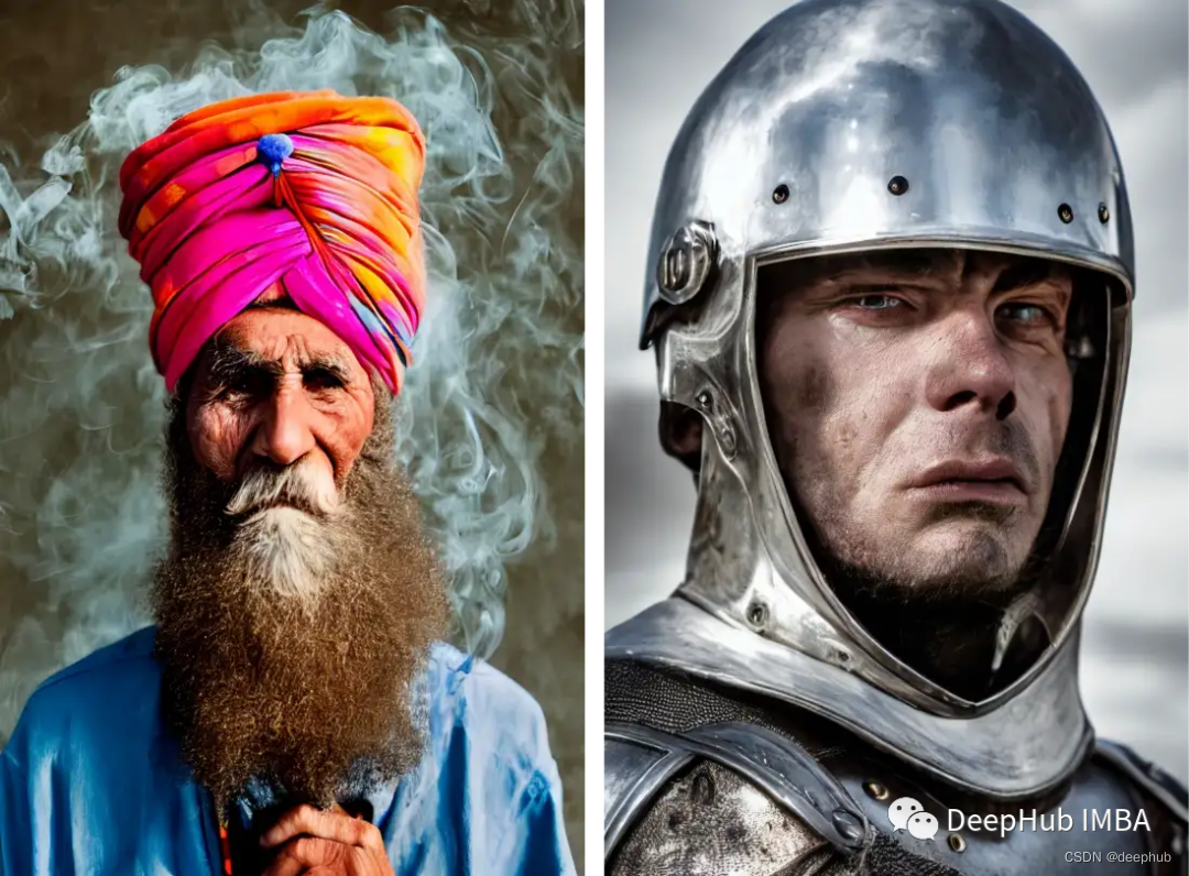
如果你足够聪明和有创造力，你可以创造一系列的图像，然后形成一个视频。例如，Xander Steenbrugge使用它和上图所示的输入提示创建了下面这段令人惊叹的《穿越时间》视频。

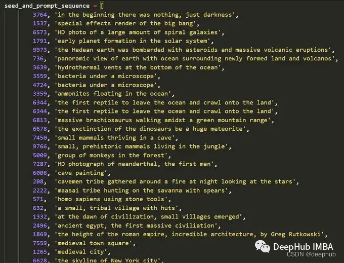
以下是他用来创作这幅创造性艺术作品的灵感和文本:

本文首先介绍什么是Stable Diffusion，并讨论它的主要组成部分。然后我们将使用模型以三种不同的方式创建图像，这三种方式从更简单到复杂。

Stable Diffusion

Stable Diffusion是一种机器学习模型，它经过训练可以逐步对随机高斯噪声进行去噪以获得感兴趣的样本，例如生成图像。

扩散模型有一个主要的缺点就是去噪过程的时间和内存消耗都非常昂贵。这会使进程变慢，并消耗大量内存。主要原因是它们在像素空间中运行，特别是在生成高分辨率图像时。

Latent diffusion通过在较低维度的潜空间上应用扩散过程而不是使用实际的像素空间来减少内存和计算成本。所以Stable Diffusion引入了Latent diffusion的方式来解决这一问题计算代价昂贵的问题。

1、Latent diffusion的主要组成部分

Latent diffusion有三个主要组成部分:

自动编码器(VAE)

自动编码器(VAE)由两个主要部分组成:编码器和解码器。编码器将把图像转换成低维的潜在表示形式，该表示形式将作为下一个组件U_Net的输入。解码器将做相反的事情，它将把潜在的表示转换回图像。

在Latent diffusion训练过程中，利用编码器获得正向扩散过程中输入图像的潜表示(latent)。而在推理过程中，VAE解码器将把潜信号转换回图像。

U-Net

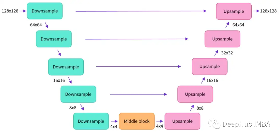
U-Net也包括编码器和解码器两部分，两者都由ResNet块组成。编码器将图像表示压缩为低分辨率图像，解码器将低分辨率解码回高分辨率图像。

为了防止U-Net在下采样时丢失重要信息，通常在编码器的下采样的ResNet和解码器的上采样ResNet之间添加了捷径的连接。

在Stable Diffusion的U-Net中添加了交叉注意层对文本嵌入的输出进行调节。交叉注意层被添加到U-Net的编码器和解码器ResNet块之间。

Text-Encoder

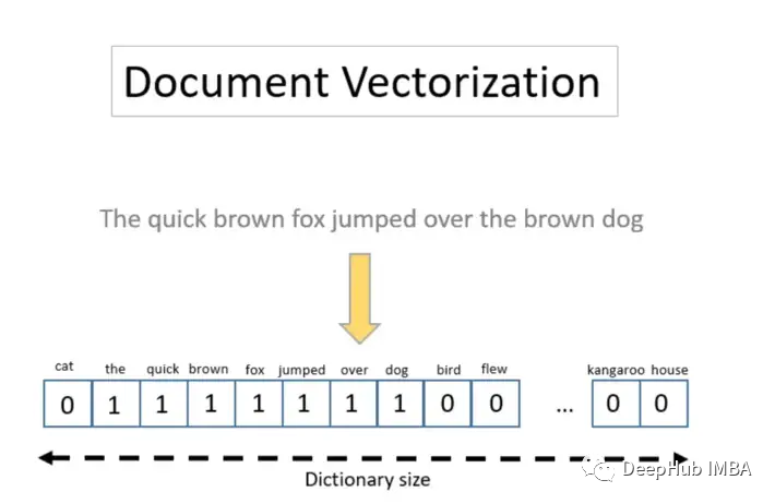
文本编码器将把输入文字提示转换为U-Net可以理解的嵌入空间，这是一个简单的基于transformer的编码器，它将标记序列映射到潜在文本嵌入序列。从这里可以看到使用良好的文字提示以获得更好的预期输出。

为什么Latent Diffusion快速有效

Latent Diffusion之所以快速有效，是因为它的U-Net是在低维空间上工作的。与像素空间扩散相比，这降低了内存和计算复杂度。例如，一个(3,512,512)的图像在潜在空间中会变成(4,64,64)，内存将会减少64倍。

Stable Diffusion的推理过程

首先，模型将潜在空间的随机种子和文本提示同时作为输入。然后使用潜在空间的种子生成大小为64×64的随机潜在图像表示，通过CLIP的文本编码器将输入的文本提示转换为大小为77×768的文本嵌入。

然后，使用U-Net 在以文本嵌入为条件的同时迭代地对随机潜在图像表示进行去噪。 U-Net 的输出是噪声的残差，用于通过scheduler 程序算法计算去噪的潜在图像表示。 scheduler 算法根据先前的噪声表示和预测的噪声残差计算预测的去噪图像表示。

许多不同的scheduler 算法可以用于这个计算，每一个都有它的优点和缺点。对于Stable Diffusion，建议使用以下其中之一:

• PNDM scheduler (默认)
• DDIM scheduler
• K-LMS scheduler

去噪过程重复约50次，这样可以逐步检索更好的潜在图像表示。一旦完成，潜在图像表示就会由变分自编码器的解码器部分进行解码。

使用 Hugging Face的API

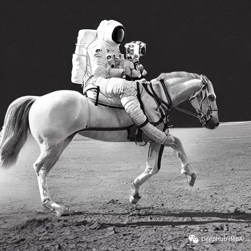
Hugging Face提供了一个非常简单的API来使用我们的模型生成图像。在下图中可以看到我使用了“astronaut riding a horse”作为输入得到输出图像:

他提供的模型还包含了一些可用的高级选项来改变生成的图像的质量，如下图所示:

这里的四个选项说明如下:

images:该选项控制的生成图像数量最多为4个。

Steps:此选项选择想要的扩散过程的步骤数。步骤越多，生成的图像质量越好。如果想要高质量，可以选择可用的最大步骤数，即50。如果你想要更快的结果，那么考虑减少步骤的数量。

Guidance Scale:Guidance Scale是生成的图像与输入提示的紧密程度与输入的多样性之间的权衡。它的典型值在7.5左右。增加的比例越多，图像的质量就会越高，但是你得到的输出就会越少。

Seed:随机种子够控制生成的样本的多样性

使用Diffuser 包

第二种使用的方法是使用Hugging Face的Diffusers库，它包含了目前可用的大部分稳定扩散模型，我们可以直接在谷歌的Colab上运行它。

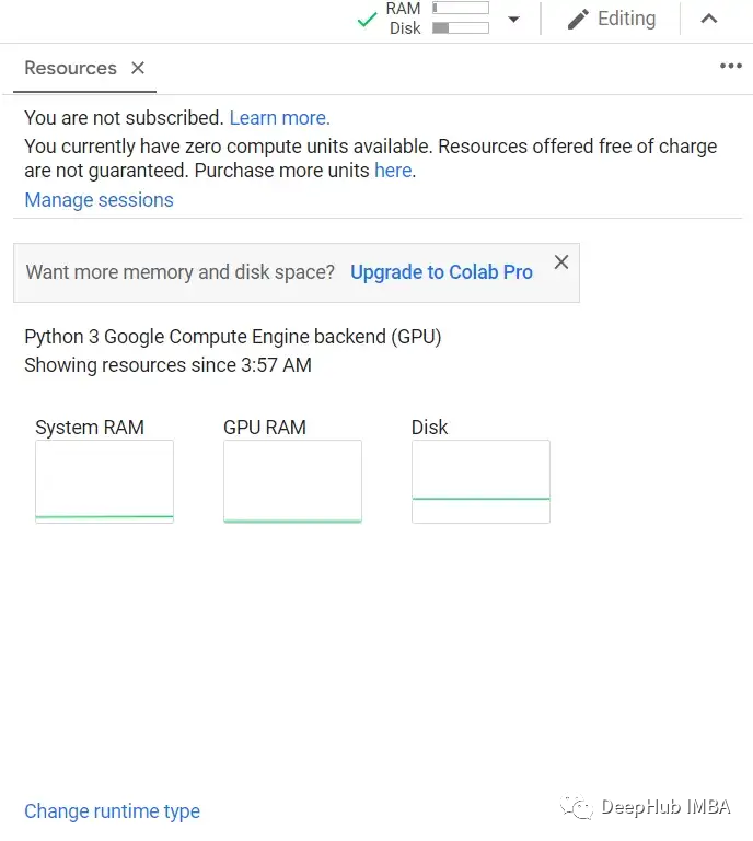
第一步是打开谷歌collab，检查是否连接到GPU，可以在资源按钮中查看，如下图所示:

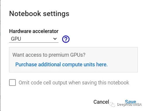
另一个选择是从运行时菜单中选择更改运行时类型，然后检查硬件加速器被选择为GPU:

我们确保使用GPU运行时后，使用下面的代码，查看我们得到的GPU

!nvidia-smi

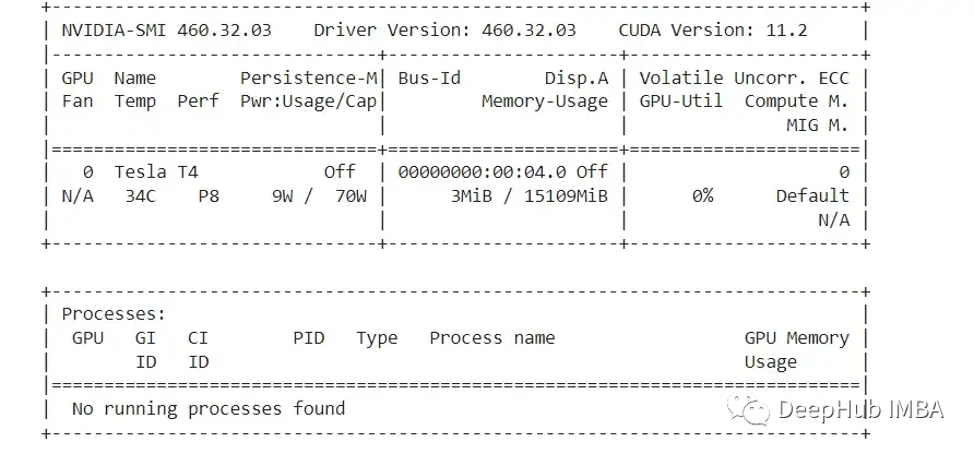
非常不幸我们只分配到了一个T4，如果你能分配到一块P100，那么你的推理速度会变得更快

下面我们安装一些需要的包：diffusers ,scipy, ftfy和transformer:

!pip install diffusers==0.4.0
!pip install transformers scipy ftfy
!pip install "ipywidgets>=7,<8"

这里需要的额外操作是必须同意模型协议，还要通过勾选复选框来接受模型许可。“Hugging Face”上注册，并获得访问令牌等等。

另外对于谷歌collab，它已经禁用了外部小部件，所以需要启用它。运行以下代码这样才能够使用“notebook_login”

from google.colab import output
output.enable_custom_widget_manager()

现在就可以从的账户中获得的访问令牌登录Hugging Face了:

from huggingface_hub import notebook_login

notebook_login()

从diffusers库加载StableDiffusionPipeline。StableDiffusionPipeline是一个端到端推理管道，可用于从文本生成图像。

我们将加载预训练模型权重。模型id将是CompVis/ stable-diffusion-v1-4，我们也将使用一个特定类型的修订版torch_dtype函数。设置revision = “fp16”从半精度分支加载权重，并设置torch_dtype = " torch。torch_dtype = “torch.float16”告诉模型使用fp16的权重

像这样设置可以减少内存，并且运行的更快。

import torch
from diffusers import StableDiffusionPipeline

# make sure you're logged in with `huggingface-cli login`
pipe = StableDiffusionPipeline.from_pretrained("CompVis/stable-diffusion-v1-4", revision="fp16", torch_dtype=torch.float16)  

下面设置GPU

pipe = pipe.to("cuda")

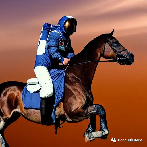
现在就可以生成图片了。我们将编写一个提示文本并将其交给管道并打印输出。这里的输入提示是“an astronaut riding a horse”，让看看输出:

prompt = "a photograph of an astronaut riding a horse"
image = pipe(prompt).images[0]  # image here is in [PIL format](https://pillow.readthedocs.io/en/stable/)

# Now to display an image you can do either save it such as:
image.save(f"astronaut_rides_horse.png")

每次运行上面的代码，都会得到不同的图像。为了每次都得到相同的结果，你可以向传递一个随机种子，如下面的代码所示:

import torch
generator = torch.Generator("cuda").manual_seed(1024)
image = pipe(prompt, generator=generator).images[0]
image

还可以使用num_inference_steps参数更改步骤的数量。一般来说，推理步骤越多，生成的图像质量越高，但生成结果需要更多的时间。如果你想要更快的结果，你可以使用更少的步骤。

下面的单元格使用与前面相同的种子，但步骤更少。注意一些细节，如马头或头盔，比前一张图定义得更模糊:

import torch
generator = torch.Generator("cuda").manual_seed(1024)
image = pipe(prompt, num_inference_steps=15, generator=generator).images[0]
image

[外链图片转存失败,源站可能有防盗链机制,建议将图片保存下来直接上传(img-1vCOAWh3-1668746176988)(http://images.overfit.cn/upload/20221118/b13d83fcbcde491796fe766a658adb9c.png)]

另一个参数是Guidance Scale。这是一种提高对条件信号的依从性的方法，在扩散模型的情况下它是文本和整体样本质量。

简单地说，无分类信息的引导迫使生成与文本提示更好地匹配。像7或8.5这样的数字可以给出很好的结果。如果使用的数字非常大图像可能看起来很好，但会减少多样性。

如果要为相同的文本提示生成多个图像，只需重复多次输入相同的文本即可。我们可以把文本的列表发送到模型中，让我们编写一个助手函数来显示多个图像

from PIL import Image

def image_grid(imgs, rows, cols):
    assert len(imgs) == rows*cols

    w, h = imgs[0].size
    grid = Image.new('RGB', size=(cols*w, rows*h))
    grid_w, grid_h = grid.size
    
    for i, img in enumerate(imgs):
        grid.paste(img, box=(i%cols*w, i//cols*h))
    return grid

现在，我们可以生成多个图像并一起展示了。

num_images = 3
prompt = ["a photograph of an astronaut riding a horse"] * num_images

images = pipe(prompt).images

grid = image_grid(images, rows=1, cols=3)
grid

[外链图片转存失败,源站可能有防盗链机制,建议将图片保存下来直接上传(img-GgiAVzsm-1668746289530)(http://images.overfit.cn/upload/20221118/620aff45e9024135bafb4b33f0c623a0.png#pic_center)]

还可以生成n*m张图像:

num_cols = 3
num_rows = 4

prompt = ["a photograph of an astronaut riding a horse"] * num_cols

all_images = []
for i in range(num_rows):
  images = pipe(prompt).images
  all_images.extend(images)

grid = image_grid(all_images, rows=num_rows, cols=num_cols)
grid

生成的图像默认大小为512*512像素。可以使用height和width参数来更改生成图像的高度和宽度。这里有一些选择好的图片大小的技巧:

将height和width参数都选择为8的倍数。高度和宽度设置为小于512,可能会导致质量比较差如果两个都设置为512以上可能会出现全局连贯性(Global Coherence)，所以如果需要大图像可以试试选一个值固定的512，而另一个大于512。例如下面的大小：

prompt = "a photograph of an astronaut riding a horse"

image = pipe(prompt, height=512, width=768).images[0]
image

建立你自己的处理管道

我们也可以通过Diffusers自定义扩散管道与扩散器。这里将演示如何使用不同的scheduler，即Katherine Crowson的K-LMS调度器。

我们先看一下StableDiffusionPipeline:

import torch
torch_device = "cuda" if torch.cuda.is_available() else "cpu"

预训练的模型包括建立一个完整的管道所需的所有组件。它们存放在以下文件夹中:

text_encoder:Stable Diffusion使用CLIP，但其他扩散模型可能使用其他编码器，如BERT。

tokenizer:它必须与text_encoder模型使用的标记器匹配。

scheduler:用于在训练过程中逐步向图像添加噪声的scheduler算法。

U-Net:用于生成输入的潜在表示的模型。

VAE，我们将使用它将潜在的表示解码为真实的图像。

可以通过引用组件被保存的文件夹，使用from_pretraining的子文件夹参数来加载组件。

from transformers import CLIPTextModel, CLIPTokenizer
from diffusers import AutoencoderKL, UNet2DConditionModel, PNDMScheduler

# 1. Load the autoencoder model which will be used to decode the latents into image space. 
vae = AutoencoderKL.from_pretrained("CompVis/stable-diffusion-v1-4", subfolder="vae")

# 2. Load the tokenizer and text encoder to tokenize and encode the text. 
tokenizer = CLIPTokenizer.from_pretrained("openai/clip-vit-large-patch14")
text_encoder = CLIPTextModel.from_pretrained("openai/clip-vit-large-patch14")

# 3. The UNet model for generating the latents.
unet = UNet2DConditionModel.from_pretrained("CompVis/stable-diffusion-v1-4", subfolder="unet")

现在，我们不加载预定义的scheduler，而是加载K-LMS

from diffusers import LMSDiscreteScheduler

scheduler = LMSDiscreteScheduler(beta_start=0.00085, beta_end=0.012, beta_schedule="scaled_linear", num_train_timesteps=1000)

将模型移动到GPU上。

vae = vae.to(torch_device)
text_encoder = text_encoder.to(torch_device)
unet = unet.to(torch_device) 

定义用于生成图像的参数。与前面的示例相比，设置num_inference_steps = 100来获得更明确的图像。

prompt = ["a photograph of an astronaut riding a horse"]

height = 512                        # default height of Stable Diffusion
width = 512                         # default width of Stable Diffusion

num_inference_steps = 100            # Number of denoising steps

guidance_scale = 7.5                # Scale for classifier-free guidance

generator = torch.manual_seed(32)   # Seed generator to create the inital latent noise

batch_size = 1

获取文本提示的text_embeddings。然后将嵌入用于调整U-Net模型。

text_input = tokenizer(prompt, padding="max_length", max_length=tokenizer.model_max_length, truncation=True, return_tensors="pt")

with torch.no_grad():
  text_embeddings = text_encoder(text_input.input_ids.to(torch_device))[0]

获得用于无分类器引导的无条件文本嵌入，这只是填充令牌(空文本)的嵌入。它们需要具有与text_embeddings (batch_size和seq_length)相同的形状。

max_length = text_input.input_ids.shape[-1]
uncond_input = tokenizer(
    [""] * batch_size, padding="max_length", max_length=max_length, return_tensors="pt"
)
with torch.no_grad():
  uncond_embeddings = text_encoder(uncond_input.input_ids.to(torch_device))[0] 

对于无分类的引导，需要进行两次向前传递。第一个是条件输入(text_embeddings)，第二个是无条件嵌入(uncond_embeddings)。把两者连接到一个批处理中，以避免进行两次向前传递:

text_embeddings = torch.cat([uncond_embeddings, text_embeddings])

生成初始随机噪声:

latents = torch.randn(
  (batch_size, unet.in_channels, height // 8, width // 8),
  generator=generator,
)
latents = latents.to(torch_device)

产生的形状为64 * 64的随机潜在空间。模型会将这种潜在的表示(纯噪声)转换为512 * 512的图像。

使用所选的num_inference_steps初始化scheduler。这将计算sigma和去噪过程中使用的确切步长值:

scheduler.set_timesteps(num_inference_steps)

K-LMS需要用它的sigma值乘以潜在空间的值:

latents = latents * scheduler.init_noise_sigma

最后就是去噪的循环:

from tqdm.auto import tqdm
from torch import autocast

for t in tqdm(scheduler.timesteps):
  # expand the latents if we are doing classifier-free guidance to avoid doing two forward passes.
  latent_model_input = torch.cat([latents] * 2)

  latent_model_input = scheduler.scale_model_input(latent_model_input, t)

  # predict the noise residual
  with torch.no_grad():
    noise_pred = unet(latent_model_input, t, encoder_hidden_states=text_embeddings).sample

  # perform guidance
  noise_pred_uncond, noise_pred_text = noise_pred.chunk(2)
  noise_pred = noise_pred_uncond + guidance_scale * (noise_pred_text - noise_pred_uncond)

  # compute the previous noisy sample x_t -> x_t-1
  latents = scheduler.step(noise_pred, t, latents).prev_sample

然后就是使用vae可将产生的潜在空间解码回图像:

# scale and decode the image latents with vae
latents = 1 / 0.18215 * latents

with torch.no_grad():
  image = vae.decode(latents).sample

最后将图像转换为PIL，以便我们可以显示或保存它。

image = (image / 2 + 0.5).clamp(0, 1)
image = image.detach().cpu().permute(0, 2, 3, 1).numpy()
images = (image * 255).round().astype("uint8")
pil_images = [Image.fromarray(image) for image in images]
pil_images[0]

这样一个完整的Stable Diffusion模型的处理过程就完成了。看完本文希望你已经知道了如何使用Stable Diffusion以及它具体工作的原理，如果你对他的处理流程还有疑问，可以通过自定义处理管道来深入的了解他的工作流程，希望本文对你有所帮助。

如果你对本文感兴趣 代码在这里：
https://avoid.overfit.cn/post/b4dfff8d1d1a4808a296c33b2e8a952b

作者：Youssef Hosni