地理加权回归（GWR）

GWR本质上是一种局部加权回归模型，GWR根据每个空间对象的周围信息，逐个对象建立起回归方程，即每个对象都有自己的回归方程，可用于归因或者对未来的预测。GWR最大的优势是考虑了空间对象的局部效应

本实验基于GWR官网提供的Georgia数据，美国佐治亚州受教育程度及各因素的空间差异性进行分析

数据下载地址： https://sgsup.asu.edu/sparc/mgwr

author：jiangroubao

date：2021-5-21

导入包

import numpy as np
import libpysal as ps
from mgwr.gwr import GWR, MGWR
from mgwr.sel_bw import Sel_BW
import geopandas as gp
import matplotlib.pyplot as plt
import matplotlib as mpl
import pandas as pd

data_dir="/home/lighthouse/Learning/pysal/data/"

导入数据

georgia_data = pd.read_csv(data_dir+"GData_utm.csv")
georgia_shp = gp.read_file(data_dir+'G_utm.shp')

查看数据概况

数据共有13个字段，其含义分别是：

AreaKey：地区代码
TotPop90：1990年人口数量
PctRural：乡村人口占比
PctBach：本科以上人口占比
PctEld：老龄人口占比
PctFB：外国出生人口占比
PctPov：贫困人口占比
PctBlack：非洲裔美国人占比
ID：地区ID
Latitude：纬度（地理坐标系）
Longitud：经度（地理坐标系）
X：投影坐标系X坐标
Y：投影坐标系Y坐标

georgia_data.head()

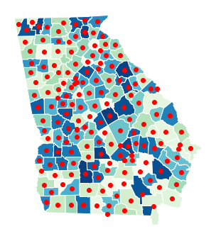
绘制分布概况

ax = georgia_shp.plot(edgecolor='white',column="AreaKey",cmap='GnBu',figsize=(6,6))
georgia_shp.centroid.plot(ax=ax, color='r',marker='o')
ax.set_axis_off()

准备输入GWR中的变量

因变量：PctBach（本科以上人口占比）作为
自变量：TotPop90（1990年总人口）、PctRural（农村人口占比）、PctEld（老年人口占比）、PctFB（外国人口出生占比）、PctPov（生活在贫困线以下居民占比）、PctBlack（非裔美国人占比）

# 因变量
g_y = georgia_data['PctBach'].values.reshape((-1,1))

# 自变量
g_X = georgia_data[['TotPop90','PctRural','PctEld','PctFB','PctPov','PctBlack']].values

# 坐标信息Latitude	Longitud
u = georgia_data['Longitud']
v = georgia_data['Latitude']
g_coords = list(zip(u,v))

# z标准化
# g_X = (g_X - g_X.mean(axis=0)) / g_X.std(axis=0)
# g_y = g_y.reshape((-1,1))
# g_y = (g_y - g_y.mean(axis=0)) / g_y.std(axis=0)

GWR模型拟合

# 带宽选择函数
gwr_selector = Sel_BW(g_coords, g_y, g_X)
gwr_bw = gwr_selector.search(search_method='golden_section',criterion='AICc')
print('最佳带宽大小为：',gwr_bw)

最佳带宽大小为： 151.0

# GWR拟合
gwr_results = GWR(g_coords, g_y, g_X, gwr_bw, fixed=False, kernel='bisquare', constant=True, spherical=True).fit()

输出GWR拟合结果

gwr_results.summary()

===========================================================================
Model type                                                         Gaussian
Number of observations:                                                 159
Number of covariates:                                                     7

Global Regression Results
---------------------------------------------------------------------------
Residual sum of squares:                                           1816.164
Log-likelihood:                                                    -419.240
AIC:                                                                852.479
AICc:                                                               855.439
BIC:                                                               1045.690
R2:                                                                   0.646
Adj. R2:                                                              0.632

Variable                              Est.         SE  t(Est/SE)    p-value
------------------------------- ---------- ---------- ---------- ----------
X0                                  14.777      1.706      8.663      0.000
X1                                   0.000      0.000      4.964      0.000
X2                                  -0.044      0.014     -3.197      0.001
X3                                  -0.062      0.121     -0.510      0.610
X4                                   1.256      0.310      4.055      0.000
X5                                  -0.155      0.070     -2.208      0.027
X6                                   0.022      0.025      0.867      0.386

Geographically Weighted Regression (GWR) Results
---------------------------------------------------------------------------
Spatial kernel:                                           Adaptive bisquare
Bandwidth used:                                                     151.000

Diagnostic information
---------------------------------------------------------------------------
Residual sum of squares:                                           1499.592
Effective number of parameters (trace(S)):                           13.483
Degree of freedom (n - trace(S)):                                   145.517
Sigma estimate:                                                       3.210
Log-likelihood:                                                    -404.013
AIC:                                                                836.992
AICc:                                                               840.117
BIC:                                                                881.440
R2:                                                                   0.708
Adjusted R2:                                                          0.680
Adj. alpha (95%):                                                     0.026
Adj. critical t value (95%):                                          2.248

Summary Statistics For GWR Parameter Estimates
---------------------------------------------------------------------------
Variable                   Mean        STD        Min     Median        Max
-------------------- ---------- ---------- ---------- ---------- ----------
X0                       15.043      1.455     12.234     15.907     16.532
X1                        0.000      0.000      0.000      0.000      0.000
X2                       -0.041      0.011     -0.062     -0.039     -0.025
X3                       -0.174      0.046     -0.275     -0.171     -0.082
X4                        1.466      0.703      0.489      1.495      2.445
X5                       -0.095      0.069     -0.206     -0.094      0.001
X6                        0.010      0.033     -0.039      0.002      0.076
===========================================================================

拟合参数空间化

# 回归参数
var_names=['cof_Intercept','cof_TotPop90','cof_PctRural','cof_PctEld','cof_PctFB','cof_PctPov','cof_PctBlack']
gwr_coefficent=pd.DataFrame(gwr_results.params,columns=var_names)

# 回归参数显著性
gwr_flter_t=pd.DataFrame(gwr_results.filter_tvals())

# 将点数据回归结果放到面上展示 
# 主要是由于两个文件中的记录数不同，矢量面中的记录比csv中多几条，因此需要将没有参加gwr的区域去掉
georgia_data_geo=gp.GeoDataFrame(georgia_data,geometry=gp.points_from_xy(georgia_data.X, georgia_data.Y))
georgia_data_geo=georgia_data_geo.join(gwr_coefficent)

# 将回归参数与面数据结合
georgia_shp_geo=gp.sjoin(georgia_shp,georgia_data_geo, how="inner", op='intersects').reset_index()

绘制回归系数分布图

fig,ax = plt.subplots(nrows=2, ncols=4,figsize=(20,10))
axes = ax.flatten()

for i in range(0,len(axes)-1):
    
    ax=axes[i]
    ax.set_title(var_names[i])
    georgia_shp_geo.plot(ax=ax,column=var_names[i],edgecolor='white',cmap='Blues',legend=True)
    
    if (gwr_flter_t[i] == 0).any():
        georgia_shp_geo[gwr_flter_t[i] == 0].plot(color='lightgrey', ax=ax, edgecolor='white') # 灰色部分表示该系数不显著
 
    
    ax.set_axis_off()
    if i+1==7:
        axes[7].axis('off')
        
plt.show()

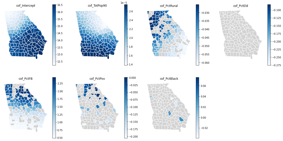
因此，从系数的分布就可以看出各个因素在每个州对于受教育程度的影响大小是不同的，并且有的因素的影响可能并不显著

参考链接

文章出处登录后可见！

已经登录？立即刷新

Python空间分析| 03 利用Python进行地理加权回归（GWR）