(1)损失函数
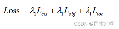
YOLOv5的损失主要由三个部分组成:
- Classes loss,分类损失,采用BCE loss,只计算正样本的分类损失。
- Objectness loss,obj置信度损失,采用BCE loss,计算的是所有样本的obj损失。注意这里的obj指的是网络预测的目标边界框与GT Box的CIoU。
- Location loss,定位损失,采用CIoU loss,只计算正样本的定位损失。
针对三个预测特征层(P3, P4, P5)上的obj损失采用不同的权重。在源码中,针对预测小目标的预测特征层(P3)采用的权重是4.0,针对预测中等目标的预测特征层(P4)采用的权重是1.0,针对预测大目标的预测特征层(P5)采用的权重是0.4。
self.balance = {3: [4.0, 1.0, 0.4]}.get(det.nl, [4.0, 1.0, 0.25, 0.06, .02])  # P3-P7
lobj += obji * self.balance[i]  # obj loss
(2)边界框计算公式(消除grid敏感度)
详情见YOLOv5网络详解
原来边界框计算公式:
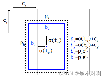
tx,ty为网络预测的目标中心点距离栅格左上点的偏移量,σ为sigmoid函数,将预测的偏移量限制在0到1之间,即预测的中心点不会超出对应的栅格区域。
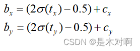
YOLOv5作者将偏移的范围由原来的( 0 , 1 )调整到了( − 0.5 , 1.5 ):
目标宽高的计算公式调整为:
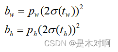
调整后倍率因子被限制在( 0 , 4 ) 之间,对预测目标的宽高做了限制。
pxy = ps[:, :2].sigmoid() * 2. - 0.5
pwh = (ps[:, 2:4].sigmoid() * 2) ** 2 * anchors[i]
pbox = torch.cat((pxy, pwh), 1)  # predicted box
(3)匹配样本方式
①:根据GT Box与对应的Anchor Templates模板的高宽比例(0.25~4)进行匹配。
②:栅格左上角点距离GT中心点在( − 0.5 , 1.5 ) 范围,它们对应的Anchor都能回归到GT的位置,这样会让正样本的数量得到大量的扩充。
损失函数的代码注释,主要参考:
class ComputeLoss:
    # Compute losses
    def __init__(self, model, autobalance=False):
        super(ComputeLoss, self).__init__()
        self.sort_obj_iou = False  # 筛选置信度损失的时候是否先对iou排序
        device = next(model.parameters()).device  # get model device
        h = model.hyp  # hyperparameters

        # Define criteria:Binary Cross Entropy
        BCEcls = nn.BCEWithLogitsLoss(pos_weight=torch.tensor([h['cls_pw']], device=device))  # 分类损失
        BCEobj = nn.BCEWithLogitsLoss(pos_weight=torch.tensor([h['obj_pw']], device=device))  # 置信度损失

        # Class label smoothing https://arxiv.org/pdf/1902.04103.pdf eqn 3
        self.cp, self.cn = smooth_BCE(eps=h.get('label_smoothing', 0.0))  # positive, negative BCE targets 1, 0

        # Focal loss
        g = h['fl_gamma']  # focal loss gamma = 0
        if g > 0:
            BCEcls, BCEobj = FocalLoss(BCEcls, g), FocalLoss(BCEobj, g)

        # det: 返回的是模型的检测头 Detector 3个 分别对应产生三个输出feature map
        det = model.module.model[-1] if is_parallel(model) else model.model[-1]  # Detect() module
        self.balance = {3: [4.0, 1.0, 0.4]}.get(det.nl, [4.0, 1.0, 0.25, 0.06, .02])  # P3-P7 预测特征层的置信度损失系数
        self.ssi = list(det.stride).index(16) if autobalance else 0  # stride 16 index    # 0
        self.BCEcls, self.BCEobj, self.gr, self.hyp, self.autobalance = BCEcls, BCEobj, 1.0, h, autobalance
        for k in 'na', 'nc', 'nl', 'anchors':
            setattr(self, k, getattr(det, k))  # 讲det的k属性赋值给self.k属性

    def __call__(self, p, targets):  # predictions, targets, model
        device = targets.device
        # 初始化lcls, lbox, lobj三种损失值  tensor([0.])
        lcls, lbox, lobj = torch.zeros(1, device=device), torch.zeros(1, device=device), torch.zeros(1, device=device)
        tcls, tbox, indices, anchors = self.build_targets(p, targets)  # targets  # 参考build_targets函数

        # Losses # 依次遍历三个feature map的预测输出pi
        for i, pi in enumerate(p):  # layer index, layer predictions
            b, a, gj, gi = indices[i]  # image, anchor, gridy, gridx
            tobj = torch.zeros_like(pi[..., 0], device=device)  # target obj # 初始化target置信度(先全是负样本 后面再筛选正样本赋值)


            n = b.shape[0]  # number of targets
            if n:
                # 精确得到b图片,a anchor,grid_cell(gi, gj)对应的预测值
                # 用这个预测值与我们筛选的这个grid_cell的真实框进行预测(计算损失)
                ps = pi[b, a, gj, gi]  # prediction subset corresponding to targets

                # Regression
                pxy = ps[:, :2].sigmoid() * 2. - 0.5
                pwh = (ps[:, 2:4].sigmoid() * 2) ** 2 * anchors[i]
                pbox = torch.cat((pxy, pwh), 1)  # predicted box
                # 这里的tbox[i]中的xy是这个target对当前grid_cell左上角的偏移量[0,1]  而pbox.T是一个归一化的值
                iou = bbox_iou(pbox.T, tbox[i], x1y1x2y2=False, CIoU=True)  # iou(prediction, target)
                lbox += (1.0 - iou).mean()  # iou loss 定位损失

                # Objectness
                # iou.detach()  不会更新iou梯度  iou并不是反向传播的参数 所以不需要反向传播梯度信息
                score_iou = iou.detach().clamp(0).type(tobj.dtype)
                if self.sort_obj_iou:
                    sort_id = torch.argsort(score_iou)
                    b, a, gj, gi, score_iou = b[sort_id], a[sort_id], gj[sort_id], gi[sort_id], score_iou[sort_id]
                # self.gr是iou ratio [0, 1]  self.gr越大,置信度越接近iou  self.gr越小,置信度越接近1(人为加大训练难度)
                tobj[b, a, gj, gi] = (1.0 - self.gr) + self.gr * score_iou  # iou ratio

                # Classification
                if self.nc > 1:  # cls loss (only if multiple classes)
                    t = torch.full_like(ps[:, 5:], self.cn, device=device)  # targets
                    t[range(n), tcls[i]] = self.cp  # 筛选到的正样本对应位置值是cp 1
                    lcls += self.BCEcls(ps[:, 5:], t)  # BCE 分类损失

                # Append targets to text file
                # with open('targets.txt', 'a') as file:
                #     [file.write('%11.5g ' * 4 % tuple(x) + '\n') for x in torch.cat((txy[i], twh[i]), 1)]

            # 置信度损失是用所有样本(正样本 + 负样本)一起计算损失的
            obji = self.BCEobj(pi[..., 4], tobj)
            lobj += obji * self.balance[i]  # obj loss 置信度损失
            if self.autobalance:
                self.balance[i] = self.balance[i] * 0.9999 + 0.0001 / obji.detach().item()

        if self.autobalance:
            self.balance = [x / self.balance[self.ssi] for x in self.balance]
        lbox *= self.hyp['box']
        lobj *= self.hyp['obj']
        lcls *= self.hyp['cls']
        bs = tobj.shape[0]  # batch size

        return (lbox + lobj + lcls) * bs, torch.cat((lbox, lobj, lcls)).detach()

    def build_targets(self, p, targets):
        # Build targets for compute_loss(), input targets(image,class,x,y,w,h)
        """
        Build targets for compute_loss()
        params p:  p[i]的作用只是得到每个feature map的shape
                   预测框由模型构建中的三个检测头Detector返回的三个yolo层的输出
                   tensor格式list列表 存放三个tensor 对应的是三个yolo层的输出
                   如: [4, 3, 80, 80, 7]、[4, 3, 40, 40, 7]、[40, 3, 20, 20, 7]
                   [bs, anchor_num, grid_h, grid_w, xywh+class置信度+classes某一类别对应概率]
                   可以看出来这里的预测值p是三个yolo层每个grid_cell(每个grid_cell有三个预测值)的预测值,后面肯定要进行正样本筛选
        params targets: 数据增强后的真实框 [2, 6] [num_target,  image_index+class+xywh] xywh为归一化后的框

        return  tcls: 表示这个target所属的class index
                tbox: xywh 其中xy为这个target对当前grid_cell左上角的偏移量
                indices: b: 表示这个target属于的image index
                         a: 表示这个target使用的anchor index
                        gj: 经过筛选后确定某个target在某个网格中进行预测(计算损失)  gj表示这个网格的左上角y坐标
                        gi: 表示这个网格的左上角x坐标
                anch: 表示这个target所使用anchor的尺度(相对于这个feature map)  注意可能一个target会使用大小不同anchor进行计算
        """
        #此处为自己设置的targets
        # target = torch.tensor([[0.00000, 1.00000, 0.54517, 0.33744, 0.06395, 0.02632],
        #                        [1.00000, 0.00000, 0.96964, 0.42483, 0.06071, 0.05264]])
        na, nt = self.na, targets.shape[0]  # number of anchors 3, targets 我们这里设为2进行debug,如上
        tcls, tbox, indices, anch = [], [], [], []
        gain = torch.ones(7, device=targets.device)  # normalized to gridspace gain  tensor([1., 1., 1., 1., 1., 1., 1.])
        ai = torch.arange(na, device=targets.device).float().view(na, 1).repeat(1, nt)  # same as .repeat_interleave(nt)
        # tensor([[0., 0.],
                # [1., 1.],
                # [2., 2.]])
        # 一个特征图对应3个anchor, 将target复制3份并在后面添加anchor索引,表示当前target对应哪个anchor
        targets = torch.cat((targets.repeat(na, 1, 1), ai[:, :, None]), 2)  # append anchor indices
        # targets:  tensor([[[0.0000, 1.0000, 0.5452, 0.3374, 0.0640, 0.0263, 0.0000],
                    #        [1.0000, 0.0000, 0.9696, 0.4248, 0.0607, 0.0526, 0.0000]],

                    #        [[0.0000, 1.0000, 0.5452, 0.3374, 0.0640, 0.0263, 1.0000],
                    #        [1.0000, 0.0000, 0.9696, 0.4248, 0.0607, 0.0526, 1.0000]],

                    #        [[0.0000, 1.0000, 0.5452, 0.3374, 0.0640, 0.0263, 2.0000],
                    #        [1.0000, 0.0000, 0.9696, 0.4248, 0.0607, 0.0526, 2.0000]]])

        g = 0.5  # bias
        off = torch.tensor([[0, 0],
                            [1, 0], [0, 1], [-1, 0], [0, -1],  # j,k,l,m
                            # [1, 1], [1, -1], [-1, 1], [-1, -1],  # jk,jm,lk,lm
                            ], device=targets.device).float() * g  # offsets
        # tensor([[ 0.0000,  0.0000],
                # [ 0.5000,  0.0000],
                # [ 0.0000,  0.5000],
                # [-0.5000,  0.0000],
                # [ 0.0000, -0.5000]])

        # 遍历三个feature map,为target筛选anchor正样本
        for i in range(self.nl): # self.nl: number of detection layers   Detect的个数 = 3
            anchors = self.anchors[i]
        # 假设anchors = torch.tensor([[1.25000, 1.62500],  anchor1
                                    # [2.00000, 3.75000],  anchor2
                                    # [4.12500, 2.87500]]) anchor3
            gain[2:6] = torch.tensor(p[i].shape)[[3, 2, 3, 2]]  # xyxy gain
            # gain = torch.tensor([ 1.,  1., 20., 20., 20., 20.,  1.]) 假设现在是在20*20大小的特征图上进行预测

            # Match targets to anchors
            t = targets * gain #将target中的xywh归一化尺度放大到当前feature map的坐标尺度, x,y,w,h都乘以20
            if nt:
                # Matches
                r = t[:, :, 4:6] / anchors[:, None]  # wh ratio
        #         r:  tensor([[[1.0232, 0.3239],  target0与anchor0的宽高比 1.0232=target0的宽度/anchor0的宽度
                            #  [0.9714, 0.6479]], target1与anchor0的宽高比

                            # [[0.6395, 0.1404],  target0与anchor1的宽高比
                            #  [0.6071, 0.2807]], target1与anchor1的宽高比

                            # [[0.3101, 0.1831],   target0与anchor2的宽高比
                            #  [0.2944, 0.3662]]]) target1与anchor2的宽高比

                j = torch.max(r, 1. / r).max(2)[0] < self.hyp['anchor_t']  # compare 宽度和高度方向差异最大的值与设定值的比较
                #   tensor([[ True,  True], 第一个True表示target0与anchor0最大的宽高比<设定值 第一个True表示target1与anchor0最大的宽高比<设定值
                #           [False,  True],
                #           [False,  True]])
                # 最后的结果target0分给anchor0,target1分给anchor0,anchor1,anchor2

                t = t[j]  # filter
                # t:  tensor([[ 0.0000,  1.0000, 10.9034,  6.7488,  1.2790,  0.5264,  0.0000],
                #             [ 1.0000,  0.0000, 19.3928,  8.4966,  1.2142,  1.0528,  0.0000],
                #             [ 1.0000,  0.0000, 19.3928,  8.4966,  1.2142,  1.0528,  1.0000],
                #             [ 1.0000,  0.0000, 19.3928,  8.4966,  1.2142,  1.0528,  2.0000]])

                # Offsets
                gxy = t[:, 2:4]  # grid xy  # 相对feature map左上角的目标
                gxi = gain[[2, 3]] - gxy  # inverse  # 相对feature map右下角的目标
                j, k = ((gxy % 1. < g) & (gxy > 1.)).T  # 如gxy%1<0.5,就表示其小数部分<0.5,则更靠近左上,并且忽略第一行和第一列的格子
                l, m = ((gxi % 1. < g) & (gxi > 1.)).T  # 如gxi%1<0.5,就表示gxy的小数部分>0.5,靠近右下,并忽略最后一行和最后一列的格子
                j = torch.stack((torch.ones_like(j), j, k, l, m))
                # tensor([[ True,  True,  True,  True],
                        # [False,  True,  True,  True],  j如果是True表示当前target中心点所在的格子的左边格子也对该target进行回归(后续进行计算损失)
                        # [False,  True,  True,  True],  k如果是True表示当前target中心点所在的格子的上边格子也对该target进行回归(后续进行计算损失)
                        # [ True, False, False, False],  l如果是True表示当前target中心点所在的格子的右边格子也对该target进行回归(后续进行计算损失)
                        # [ True, False, False, False]]) m如果是True表示当前target中心点所在的格子的右边格子也对该target进行回归(后续进行计算损失)
                t = t.repeat((5, 1, 1))[j]
                # t:  tensor([[ 0.0000,  1.0000, 10.9034,  6.7488,  1.2790,  0.5264,  0.0000],
                #             [ 1.0000,  0.0000, 19.3928,  8.4966,  1.2142,  1.0528,  0.0000],
                #             [ 1.0000,  0.0000, 19.3928,  8.4966,  1.2142,  1.0528,  1.0000],
                #             [ 1.0000,  0.0000, 19.3928,  8.4966,  1.2142,  1.0528,  2.0000],
                #             [ 1.0000,  0.0000, 19.3928,  8.4966,  1.2142,  1.0528,  0.0000],
                #             [ 1.0000,  0.0000, 19.3928,  8.4966,  1.2142,  1.0528,  1.0000],
                #             [ 1.0000,  0.0000, 19.3928,  8.4966,  1.2142,  1.0528,  2.0000],
                #             [ 1.0000,  0.0000, 19.3928,  8.4966,  1.2142,  1.0528,  0.0000],
                #             [ 1.0000,  0.0000, 19.3928,  8.4966,  1.2142,  1.0528,  1.0000],
                #             [ 1.0000,  0.0000, 19.3928,  8.4966,  1.2142,  1.0528,  2.0000],
                #             [ 0.0000,  1.0000, 10.9034,  6.7488,  1.2790,  0.5264,  0.0000],
                #             [ 0.0000,  1.0000, 10.9034,  6.7488,  1.2790,  0.5264,  0.0000]])
                '''
                对t复制5份,即本身点外加上下左右四个候选区共五个区域,选出三份
                具体选出哪三份由torch.stack后的j决定,第一项是torch.ones_like,即全1矩阵,说明本身是必选中状态的。
                剩下的4项中,由于是inverse操作,所以j和l,k和m是两两互斥的。
                '''
                offsets = (torch.zeros_like(gxy)[None] + off[:, None])[j]
                # offsets tensor([[ 0.0000,  0.0000],
                #                 [ 0.0000,  0.0000],
                #                 [ 0.0000,  0.0000],
                #                 [ 0.0000,  0.0000],
                #                 [ 0.5000,  0.0000],
                #                 [ 0.5000,  0.0000],
                #                 [ 0.5000,  0.0000],
                #                 [ 0.0000,  0.5000],
                #                 [ 0.0000,  0.5000],
                #                 [ 0.0000,  0.5000],
                #                 [-0.5000,  0.0000],
                #                 [ 0.0000, -0.5000]])


            else:
                t = targets[0]
                offsets = 0

            # Define
            b, c = t[:, :2].long().T  # image, class
            gxy = t[:, 2:4]  # grid xy
            gwh = t[:, 4:6]  # grid wh
            gij = (gxy - offsets).long()
            gi, gj = gij.T  # grid xy indices

            # Append
            a = t[:, 6].long()  # anchor indices
            indices.append((b, a, gj.clamp_(0, gain[3] - 1), gi.clamp_(0, gain[2] - 1)))  # image, anchor, grid indices gj: 网格的左上角y坐标  gi: 网格的左上角x坐标
            tbox.append(torch.cat((gxy - gij, gwh), 1))  # box:xywh,其中xy为这个target对当前grid_cell左上角的偏移量,0~1之间
            anch.append(anchors[a])  # anchors
            tcls.append(c)  # class

        return tcls, tbox, indices, anch
文章出处登录后可见!
已经登录?立即刷新