YOLOv5介绍
YOLOv5为兼顾速度与性能的目标检测算法。笔者将在近期更新一系列YOLOv5的代码导读博客。YOLOv5为2021.1.5日发布的4.0版本。
YOLOv5开源项目github网址
源代码指南摘要 URL
本博客导读的代码为utils文件夹下的loss.py,取自2020。5.10更新版本。
在介绍损失函数的代码实现之前,首先介绍所使用的BCE loss: Binary Cross Entropy loss 二分类交叉熵损失函数和Focal loss的定义及对应的公式。
Binary Cross Entropy loss 二分类交叉熵损失函数(BCE)
交叉熵损失函数用于衡量样本分类的准确率,其表达式如下图所示: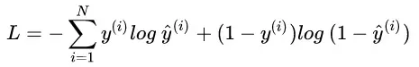
其中y尖代表模型预测第i个样本是某一类的概率,yi代表标签,因此对标签为0或1有不同的计算方式。当用于多分类问题时,其实相当于是扩充了标签本身维数,对将多个类的二进制表示写在一起构成了一个one hot向量。
为了解决类别不均衡的问题,引入alpha参数作为一个因子,对每一类的loss值做一个加权。
为了让BCEloss更具有泛化性,Kaiming He et.al 提出了Focal loss,其表达式如下所示: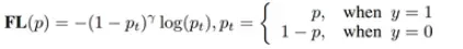
通过引入另一个超参gamma,将概率较高的正样本和概率较低的负样本的loss值显著降低了,因此难样本会对损失函数值有较大的贡献度,使得模型提高对较难样本进行区分
2020年NIPS《Generalized Focal loss》中,提出了QFocal loss,如下所示: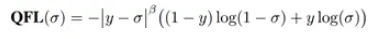
该式将每一张图片对应的概率看做是图片对应的质量,从0-1进行取值,标签中的0(不属于该类)和1(属于该类)即代表了质量的两个极端。实践中,beta取2为最佳。
loss.py
该文件给出了YOLOv5 模型中使用到的全部损失函数的定义,并提供了基于ground truth 和模型预测输出之间计算损失函数的接口。
以下为该文件必须导入的模块,其中bbox_iou和is_parallel函数来自于其他文件的定义。详细解读可以参考笔者其他博客。
import torch #pytorch 模块
import torch.nn as nn

from utils.general import bbox_iou   # bbox_iou函数详细解析见general.py文件中 该函数为返回一个box对一组box的iou值
from utils.torch_utils import is_parallel # 判断模型是否并行处理
以下是标签平滑的部分代码
# BCE: Binary Cross Entropy 二分类交叉熵损失函数 用于多类别多分类问题
def smooth_BCE(eps=0.1):  # https://github.com/ultralytics/yolov3/issues/238#issuecomment-598028441最开始提出这个改进的网址
    # return positive, negative label smoothing BCE targets
    # 标签平滑操作 两个值分别代表正样本和负样本的标签取值
    # 这样做的目的是为了后续的的 BCE loss
    return 1.0 - 0.5 * eps, 0.5 * eps
正负样本加权的BCE loss定义
class BCEBlurWithLogitsLoss(nn.Module): #blur 意为模糊 据下行原版注释是减少了错失标签带来的影响
    # BCEwithLogitLoss() with reduced missing label effects.
    def __init__(self, alpha=0.05):
        super(BCEBlurWithLogitsLoss, self).__init__()
        # 这里BCEWithLogitsLoss 是输入的每一个元素带入sigmoid函数之后 再同标签计算BCE loss
        self.loss_fcn = nn.BCEWithLogitsLoss(reduction='none')  # must be nn.BCEWithLogitsLoss()
        self.alpha = alpha #这个应该算是一个模糊系数吧 默认为0.05

    def forward(self, pred, true):
        # 得到了预测值和标签值得BCE loss 注:预测是经过sigmoid函数处理再计算BCE的
        loss = self.loss_fcn(pred, true)
        # 将预测值进行sigmoid处理 数学意义为每一位对应类别出现的概率
        pred = torch.sigmoid(pred)  # prob from logits
        # 假定missing的标签用一行0进行补齐,则相减之后missing的样本概率不受影响,正常样本样本概率为绝对值较小的负数
        dx = pred - true  # reduce only missing label effects
        """
        torch.exp()函数就是求e的多少次方  输入tensor每一个元素经过计算之后返回对应的tensor
        根据下式 对于正常的较大概率的样本 dx对应值为绝对值较小一个负数 假设为-0.12,则-1为-1.12除0.05 为-22.4,
        -22.4 指数化之后为一个很小很小的正数,1-该正数之后得到的值较大 再在loss中乘上之后影响微乎其微
        而对于missing的样本 dx对应为一个稍大的正数 如0.3 减去1之后为-0.7 除以0.05 为 -14
        -14相比-22.4值为指数级增大,因此对应的alpha_factor相比正常样本显著减小 在loss中较小考虑
        """
        # Q:有一个问题,为什么yolov5要对missing的样本有这样的容忍度,而不是选择直接屏蔽掉对应样本呢?
        alpha_factor = 1 - torch.exp((dx - 1) / (self.alpha + 1e-4))
        loss *= alpha_factor
        return loss.mean() # 这个mean的意义应该为对一批batch中的每一个样本得到的BCE loss求均值作为返回值
Focal loss定义
class FocalLoss(nn.Module): # 这里定义了FocalLoss
    # Wraps focal loss around existing loss_fcn(), i.e. criteria = FocalLoss(nn.BCEWithLogitsLoss(), gamma=1.5)
    def __init__(self, loss_fcn, gamma=1.5, alpha=0.25):
        super(FocalLoss, self).__init__()
        self.loss_fcn = loss_fcn  # must be nn.BCEWithLogitsLoss() 这里的loss_fcn基础定义为多分类交叉熵损失函数
        self.gamma = gamma  # Focal loss中的gamma参数 用于削弱简单样本对loss的贡献程度
        self.alpha = alpha  # Focal loss中的alpha参数 用于平衡正负样本个数不均衡的问题
        self.reduction = loss_fcn.reduction
        self.loss_fcn.reduction = 'none'  # 需要将Focal loss应用于每一个样本之中

    def forward(self, pred, true):
        loss = self.loss_fcn(pred, true) # 这里的loss代表正常的BCE loss结果

        # TF implementation https://github.com/tensorflow/addons/blob/v0.7.1/tensorflow_addons/losses/focal_loss.py
        # 通过sigmoid函数返回得到的概率 即Focal loss 中的y'
        pred_prob = torch.sigmoid(pred)
        # 这里对p_t属于正样本还是负样本进行了判别,正样本对应true=1,即Focal loss中的大括号
        # 正样本时 返回pred_prob为是正样本的概率y',负样本时为1-y'
        p_t = true * pred_prob + (1 - true) * (1 - pred_prob)
        # 这里同样对alpha_factor进行了属于正样本还是负样本的判别,即Focal loss中的
        alpha_factor = true * self.alpha + (1 - true) * (1 - self.alpha)
        # 这里代表Focal loss中的指数项
        # 正样本对应(1-y')的gamma次方 负样本度对应y'的gamma次方
        modulating_factor = (1.0 - p_t) ** self.gamma
        # 返回最终的loss大tensor
        loss *= alpha_factor * modulating_factor
        # 以下几个判断代表返回loss的均值/和/本体了
        if self.reduction == 'mean':
            return loss.mean()
        elif self.reduction == 'sum':
            return loss.sum()
        else:  # 'none'
            return loss
QFocal loss的定义
class QFocalLoss(nn.Module): #来自NIPS2020的Generalized Focal loss论文 除了modulate参数定义变化之外 其余定义同Focal loss相同
    # Wraps Quality focal loss around existing loss_fcn(), i.e. criteria = FocalLoss(nn.BCEWithLogitsLoss(), gamma=1.5)
    def __init__(self, loss_fcn, gamma=1.5, alpha=0.25):
        super(QFocalLoss, self).__init__()
        self.loss_fcn = loss_fcn  # must be nn.BCEWithLogitsLoss()
        self.gamma = gamma
        self.alpha = alpha
        self.reduction = loss_fcn.reduction
        self.loss_fcn.reduction = 'none'  # required to apply FL to each element

    def forward(self, pred, true):
        loss = self.loss_fcn(pred, true)

        pred_prob = torch.sigmoid(pred)
        # 对alpha参数 对正负样本进行区分
        alpha_factor = true * self.alpha + (1 - true) * (1 - self.alpha)
        # 对比一下正常的Focal loss           (1.0 - p_t) ** self.gamma
        # Focal loss对样本预先进行了正和负的区分,而QFocal loss无视这样的区分,
        # 将pred_prob看做是样本质量 负为0 正为1 直接进行做差乘方来实现泛化
        modulating_factor = torch.abs(true - pred_prob) ** self.gamma # 这里的平方幂数为实验验证得来
        loss *= alpha_factor * modulating_factor

        if self.reduction == 'mean':
            return loss.mean()
        elif self.reduction == 'sum':
            return loss.sum()
        else:  # 'none'
            return loss
以下为Compute _loss类 为方便观看,按照类中定义的方法进行区分。
这部分是类的初始化
class ComputeLoss:
    # Compute losses
    def __init__(self, model, autobalance=False):
        super(ComputeLoss, self).__init__()
        device = next(model.parameters()).device  # 获取模型对应的设备型号
        h = model.hyp  # 超参数hyperparameters

        # Define criteria
        # 定义评价标准 cls代表类别的BCE loss obj的BCElos为判断第i个网格中的第j个box是否负责对应的object
        # 这里的pos_weight为对应的参数 在模型训练的yaml文件中可以调整
        BCEcls = nn.BCEWithLogitsLoss(pos_weight=torch.tensor([h['cls_pw']], device=device))
        BCEobj = nn.BCEWithLogitsLoss(pos_weight=torch.tensor([h['obj_pw']], device=device))

        # Class label smoothing https://arxiv.org/pdf/1902.04103.pdf eqn 3
        # 这里进行标签平滑处理 cp代表positive的标签值 cn代表negative的标签值
        self.cp, self.cn = smooth_BCE(eps=h.get('label_smoothing', 0.0))  # positive, negative BCE targets

        # Focal loss定义
        g = h['fl_gamma']  # 根据yaml文件获取focal loss的gamma参数
        if g > 0:
            BCEcls, BCEobj = FocalLoss(BCEcls, g), FocalLoss(BCEobj, g)

        # 这里的det 返回的是模型的model属性的最后一项 应该返回的是包含模型检测器的那部分 不确定
        det = model.module.model[-1] if is_parallel(model) else model.model[-1]  # Detect() module
        # self.balance和self.ssi的定义需要看模型定义的主干  det.nl 对应的是检测器输出的类别个数 P3-P7对应的是什么部分需要看模型的构建
        self.balance = {3: [4.0, 1.0, 0.4]}.get(det.nl, [4.0, 1.0, 0.25, 0.06, .02])  # P3-P7
        self.ssi = list(det.stride).index(16) if autobalance else 0  # stride 16 index

        # self.BCEcls和self.BCEobj对应的是loss self.gr变量不知道 self.hyp为从yaml文件中提取到的各种超参数 autobalance不确定 猜测和anchor有关
        self.BCEcls, self.BCEobj, self.gr, self.hyp, self.autobalance = BCEcls, BCEobj, model.gr, h, autobalance
        # setattr函数为给实例对象添加属性 这里把na nc nl 和 anchor属性全部私有化
        for k in 'na', 'nc', 'nl', 'anchors':
            setattr(self, k, getattr(det, k))
调用方法 通过模型预测和标签返回loss的值和各个loss合并后的tensor
    def __call__(self, p, targets):  # predictions, targets, model
        device = targets.device  # 确定运行的设备
        # 初始化 分类 bbx回归 和obj三种损失函数值
        lcls, lbox, lobj = torch.zeros(1, device=device), torch.zeros(1, device=device), torch.zeros(1, device=device)
        # 返回目标对应的 分类结果 bbx结果 索引 和对应的anchor 见下文build_targets函数
        tcls, tbox, indices, anchors = self.build_targets(p, targets)  # targets

        # 以下for循环内 为计算loss
        # 对不同的尺度对应的层进行遍历
        for i, pi in enumerate(p):  # i: layer index, pi: layer predictions
            # b:image索引 a:anchor的索引 gj/gi:网格的纵坐标和横坐标
            b, a, gj, gi = indices[i]
            # 初始化target object tensor中的元素全部为0
            tobj = torch.zeros_like(pi[..., 0], device=device)
            # n为返回的target数目
            n = b.shape[0]
            # 当图像中含有的target数目不为0的时候 即对一张图片的标签不为0的时候
            if n:
                # ps为同targets一致的预测子集
                ps = pi[b, a, gj, gi]

                # 计算bounding box的回归损失函数
                pxy = ps[:, :2].sigmoid() * 2. - 0.5
                pwh = (ps[:, 2:4].sigmoid() * 2) ** 2 * anchors[i]
                # 得到了预测的所有bounding box
                pbox = torch.cat((pxy, pwh), 1)
                # bbx_iou(prediction, target) 计算预测框和标签框的bbx损失值 此处强制使用CIoU loss 如果要进行更换 需改这个地方
                iou = bbox_iou(pbox.T, tbox[i], x1y1x2y2=False, CIoU=True)  # 该函数详细解析见general.py 源代码解析
                lbox += (1.0 - iou).mean()  # 对iou中每一个box对应的iou都取了平均值 计算的是所有box的平均iou loss

                # 计算anchor是否存在Object的损失函数值
                tobj[b, a, gj, gi] = (1.0 - self.gr) + self.gr * iou.detach().clamp(0).type(tobj.dtype)  # 用iou值来当比例

                # 计算Classification相关的loss
                if self.nc > 1:  # cls loss (只有在类别多于1的时候才会进行计算)
                    # 以下计算中cn和cp分别代表经过标签平滑处理之后的negative样本和positive样本对应的标签值
                    # t为标签中target所在grid对应类别 的one hot 向量格式
                    t = torch.full_like(ps[:, 5:], self.cn, device=device)
                    t[range(n), tcls[i]] = self.cp
                    lcls += self.BCEcls(ps[:, 5:], t)  # 计算多分类的Focal loss

            # 计算lobj loss 这里是指bbx中有物体的置信度
            obji = self.BCEobj(pi[..., 4], tobj)
            lobj += obji * self.balance[i]  # 得到obj loss
            # 作者添加了自动平衡功能 加入了每个框是否具有物体的置信度大小带来的影响
            if self.autobalance:
                self.balance[i] = self.balance[i] * 0.9999 + 0.0001 / obji.detach().item()

        # self.ssi参数在这里用于元素的平衡
        if self.autobalance:
            self.balance = [x / self.balance[self.ssi] for x in self.balance]

        # 以下是根据超参里面的参数 对各个损失函数进行平衡
        lbox *= self.hyp['box']
        lobj *= self.hyp['obj']
        lcls *= self.hyp['cls']
        bs = tobj.shape[0]  # bs代表batchsize

        loss = lbox + lobj + lcls
        return loss * bs, torch.cat((lbox, lobj, lcls, loss)).detach() # 返回一个batch的总损失函数值 和把各个loss cat一起的大tensor
将标签转换为便于后续计算loss的格式,整理target相关信息。
    def build_targets(self, p, targets): #将预测的格式 转化为便于计算loss的target格式

        # 为compute_loss类构建目标 输入的targets为(image,class,x,y,w,h) 应该为一维向量 代表第几张图片(在一个batch中的次序)中每一个bbx及其类别
        # na变量代表number of anchors, nt变量代表number of targets
        na, nt = self.na, targets.shape[0]
        # 初始化四个列表 代表targets的类别 bbx 索引 和 anchor位置
        tcls, tbox, indices, anch = [], [], [], []
        # 归一化为空间网格增益 即为7个1 最终代表检测的7种不同属性
        gain = torch.ones(7, device=targets.device)

        # torch.arange()函数为等间隔生成一段序列 如 torch.arange(3)的结果为[0,1,2] tensor.float()为将结果转换为浮点数
        # tensor.view(na,1)此处为将一维tensor的行转换为列且升维为二维tensor
        # tensor.repeat(1,nt)此处为每一行重复第一个元素重复nt次 因此最终的ai尺寸为[na,nt]
        ai = torch.arange(na, device=targets.device).float().view(na, 1).repeat(1, nt)  # same as .repeat_interleave(nt)

        # tensor.repeat(na,1,1)将原始一维向量在第1/2/3个维度上分别重复 na,1,1次 ai[:,:,None]将原二维tensor ai扩充至三维 且第三维为1
        # tensor.cat(tensor1,tensor2,2) 将两个三维tensor在第三个维度上面拼接到了一起
        # tensor1[1*na,nt*1,1]和tensor2[na,nt,1]的张量的第三维cat一起之后 为[na,nt,2]
        targets = torch.cat((targets.repeat(na, 1, 1), ai[:, :, None]), 2)  # append anchor indices

        g = 0.5  # bias 偏置
        # offsets 偏移量 应该是对应anchor的偏移量
        off = torch.tensor([[0, 0],
                            [1, 0], [0, 1], [-1, 0], [0, -1],  # j,k,l,m
                            # [1, 1], [1, -1], [-1, 1], [-1, -1],  # jk,jm,lk,lm
                            ], device=targets.device).float() * g  # offsets

        # 这里的nl 应该代表 number of label标签的数量
        # for 对每一个标签进行迭代
        for i in range(self.nl):
            # 调取对应索引的anchor
            anchors = self.anchors[i]
            # p指prediction 模型的预测输出 这里可以看到P至少为五维 有一个[i]的索引
            # gain[2:6] 返回一个一维向量 代表p第i的元素的第四维度数目和第三维度数目 repeat double
            gain[2:6] = torch.tensor(p[i].shape)[[3, 2, 3, 2]]  # xyxy gain

            # 匹配targets到对应的anchors
            t = targets * gain
            if nt: # 当存在target时
                # Matches
                r = t[:, :, 4:6] / anchors[:, None]  # 获取wh的比例
                j = torch.max(r, 1. / r).max(2)[0] < self.hyp['anchor_t']  # 与设定的anchor_t超参进行比较
                # j = wh_iou(anchors, t[:, 4:6]) > model.hyp['iou_t']  # iou(3,n)=wh_iou(anchors(3,2), gwh(n,2))
                t = t[j]  # 过滤 获得匹配成功的目标

                # Offsets
                # 获取每一个匹配成功的目标对应的偏移量
                # 因为YOLO核心在于通过预测偏移量得到bbx 所以此步用于对偏移量进行处理 使后续根据偏移量得到对应bbx
                gxy = t[:, 2:4]  # 获取网格的xy坐标值
                gxi = gain[[2, 3]] - gxy  # 翻转
                j, k = ((gxy % 1. < g) & (gxy > 1.)).T
                l, m = ((gxi % 1. < g) & (gxi > 1.)).T
                j = torch.stack((torch.ones_like(j), j, k, l, m))
                t = t.repeat((5, 1, 1))[j]
                offsets = (torch.zeros_like(gxy)[None] + off[:, None])[j]
            else: #不存在target时返回对应空值
                t = targets[0]
                offsets = 0

            # Define
            b, c = t[:, :2].long().T  # b,c代一个target对应的image的序号和对应的class
            gxy = t[:, 2:4]  # 网格的 xy 坐标
            gwh = t[:, 4:6]  # 网格的 wh 坐标
            gij = (gxy - offsets).long()
            gi, gj = gij.T  # 网格 xy 索引

            # 将上述得到的target的信息添加到对应list中
            a = t[:, 6].long()  # anchor 索引
            indices.append((b, a, gj.clamp_(0, gain[3] - 1), gi.clamp_(0, gain[2] - 1)))  # target对应的image, anchor, grid 索引
            tbox.append(torch.cat((gxy - gij, gwh), 1))  # target对应的box
            anch.append(anchors[a])  # target对应的anchors
            tcls.append(c)  # target对应的类别class

        return tcls, tbox, indices, anch
限于作者水平有限,有不准确和不清楚的支出,欢迎广大读者提示指正!
版权声明:本文为博主幻灵H_Ling原创文章,版权归属原作者,如果侵权,请联系我们删除!
原文链接:https://blog.csdn.net/weixin_42716570/article/details/116759811