Matplotlib 3D小红花的绘制原理

前言

在上篇博客中使用了matplotlib绘制了3D小红花，本篇博客主要介绍一下3D小红花的绘制原理。

1. 极坐标系

对于极坐标系中的一点，我们可以用极径和极角来表示，记为点，相关知识在高中时已经介绍过，这里不再赘述。
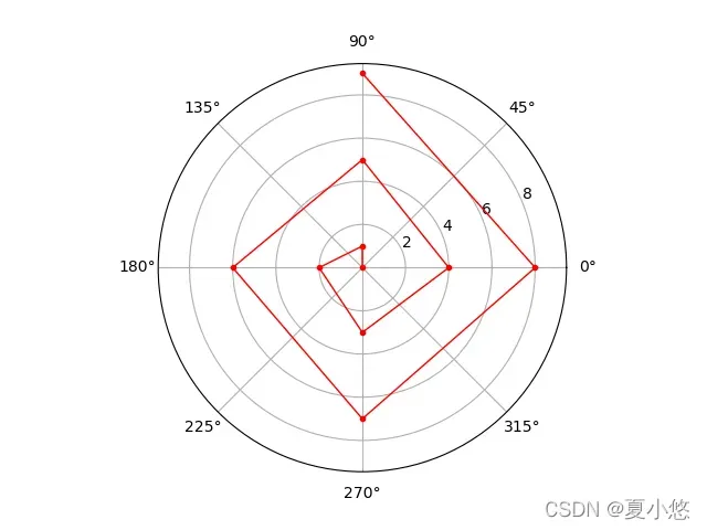
使用matplotlib绘制极坐标系：

import matplotlib.pyplot as plt
import numpy as np


if __name__ == '__main__':
    # 极径
    r = np.arange(10)
    # 角度
    theta = 0.5 * np.pi * r

    fig = plt.figure()
    plt.polar(theta, r, c='r', marker='o', ms=3, ls='-', lw=1)
    # plt.savefig('img/polar1.png')
    plt.show()

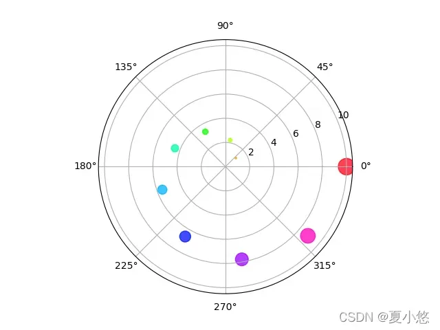
使用matplotlib绘制极坐标散点图：

import matplotlib.pyplot as plt
import numpy as np


if __name__ == '__main__':
	r = np.linspace(0, 10, num=10)
    theta = 2 * np.pi * r
    area = 3 * r ** 2

    ax = plt.subplot(111, projection='polar')
    ax.scatter(theta, r, c=theta, s=area, cmap='hsv', alpha=0.75)
    # plt.savefig('img/polar2.png')
    plt.show()

有关matplotlib极坐标的参数更多介绍，可参阅官网手册。

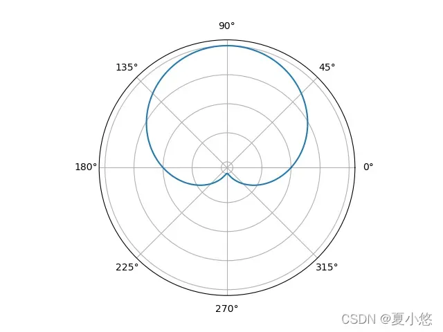
2. 极坐标系花瓣

在极坐标中绘制：

import matplotlib.pyplot as plt
import numpy as np


if __name__ == '__main__':
	fig = plt.figure()
    ax = plt.subplot(111, projection='polar')
    ax.set_rgrids(radii=np.linspace(-1, 1, num=5), labels='')

    theta = np.linspace(0, 2 * np.pi, num=200)
    r = np.sin(theta)
    ax.plot(theta, r)
    # plt.savefig('img/polar3.png')
    plt.show()

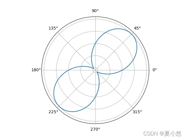
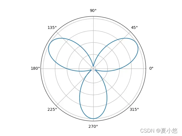
以为周期，增加图像的旋转周期：

r = np.sin(2 * theta)

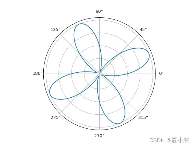
继续增加图像的旋转周期：

r = np.sin(3 * theta)
r = np.sin(4 * theta)

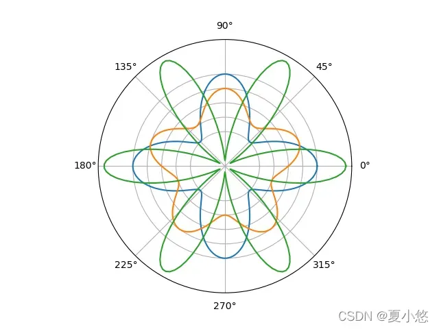
然后我们可以通过调整极径系数和角度系数来调整图像：

import matplotlib.pyplot as plt
import numpy as np


if __name__ == '__main__':
	fig = plt.figure()
    ax = plt.subplot(111, projection='polar')
    ax.set_rgrids(radii=np.linspace(-1, 1, num=5), labels='')

    theta = np.linspace(0, 2 * np.pi, num=200)
    r1 = np.sin(4 * (theta + np.pi / 8))
    r2 = 0.5 * np.sin(5 * theta)
    r3 = 2 * np.sin(6 * (theta + np.pi / 12))

    ax.plot(theta, r1)
    ax.plot(theta, r2)
    ax.plot(theta, r3)
    # plt.savefig('img/polar4.png')
    plt.show()

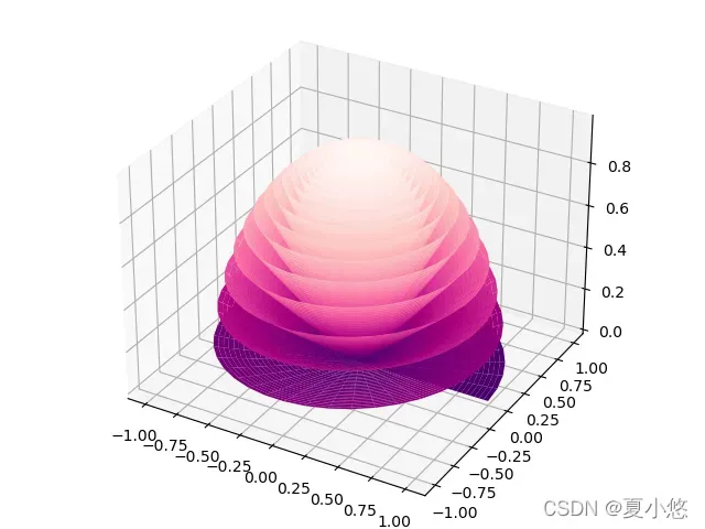
3. 三维花瓣

现在可以将花瓣放置在三维空间中。根据花瓣的生成规律，花瓣的外缘是在一个向内旋转和收缩的曲线上。 逐渐变大。
因此，我们在的基础上定义一个递减函数，保证其取值范围在内。新功能为：其功能图如下：
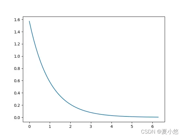
这样定义满足了前面关于花瓣外缘曲线的假设，即减小，增大。
现在把它放在 3D 空间中：

import matplotlib.pyplot as plt
import numpy as np
from mpl_toolkits.mplot3d import Axes3D


if __name__ == '__main__':
    fig = plt.figure()
    ax = Axes3D(fig)
    # plt.axis('off')

    x = np.linspace(0, 1, num=30)
    theta = np.linspace(0, 2 * np.pi, num=1200)
    theta = 30 * theta
    x, theta = np.meshgrid(x, theta)

    # f is a decreasing function of theta
    f = 0.5 * np.pi * np.exp(-theta / 50)

    r = x * np.sin(f)
    h = x * np.cos(f)

	# 极坐标转笛卡尔坐标
    X = r * np.cos(theta)
    Y = r * np.sin(theta)
    ax = ax.plot_surface(X, Y, h,
                         rstride=1, cstride=1, cmap=plt.cm.cool)

    # plt.savefig('img/polar5.png')
    plt.show()

笛卡尔坐标系(Cartesian coordinate system)，即直角坐标系。

但是，上面的表达式仍然没有得到花瓣的细节，所以我们需要在此基础上进行处理，得到花瓣的形状。因此，设计了一个花瓣函数：
是以为周期的周期函数，取值范围为。图像如下图所示：

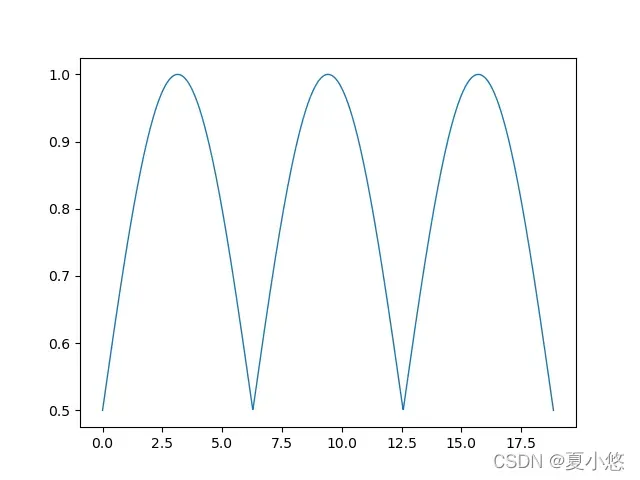
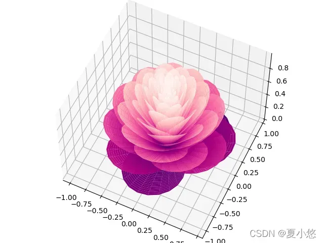
再次绘制：

import matplotlib.pyplot as plt
import numpy as np
from mpl_toolkits.mplot3d import Axes3D


if __name__ == '__main__':
	fig = plt.figure()
    ax = Axes3D(fig)
    # plt.axis('off')

    x = np.linspace(0, 1, num=30)
    theta = np.linspace(0, 2 * np.pi, num=1200)
    theta = 30 * theta
    x, theta = np.meshgrid(x, theta)

    # f is a decreasing function of theta
    f = 0.5 * np.pi * np.exp(-theta / 50)

	# 通过改变函数周期来改变花瓣的形状
	# 改变值域也可以改变花瓣形状
	# u is a periodic function
    u = 1 - (1 - np.absolute(np.sin(3.3 * theta / 2))) / 2
    r = x * u * np.sin(f)
    h = x * u * np.cos(f)
	
	# 极坐标转笛卡尔坐标
    X = r * np.cos(theta)
    Y = r * np.sin(theta)
    ax = ax.plot_surface(X, Y, h,
                         rstride=1, cstride=1, cmap=plt.cm.RdPu_r)

    # plt.savefig('img/polar6.png')
    plt.show()

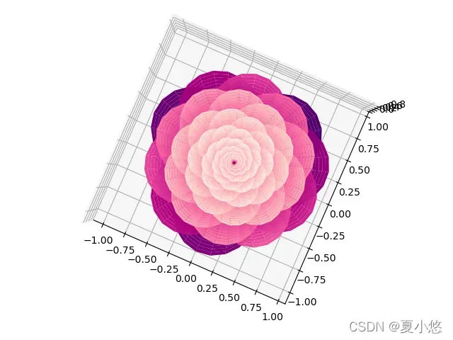
4. 花瓣微调

为了使花瓣更逼真，花瓣的形状向下凹，需要对花瓣的形状进行微调。这里，添加了校正项和噪声干扰。校正函数图像为：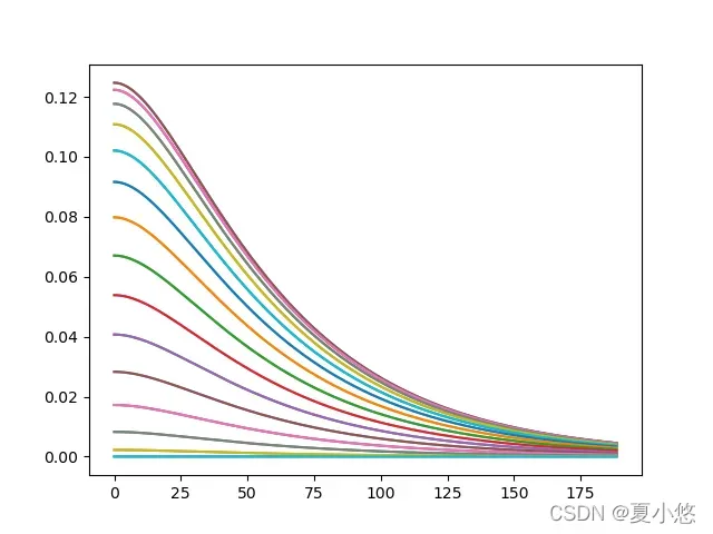

import matplotlib.pyplot as plt
import numpy as np
from mpl_toolkits.mplot3d import Axes3D


if __name__ == '__main__':
	fig = plt.figure()
    ax = Axes3D(fig)
    # plt.axis('off')

    x = np.linspace(0, 1, num=30)
    theta = np.linspace(0, 2 * np.pi, num=1200)
    theta = 30 * theta
    x, theta = np.meshgrid(x, theta)

    # f is a decreasing function of theta
    f = 0.5 * np.pi * np.exp(-theta / 50)

    noise = np.sin(theta) / 30
    # u is a periodic function
    u = 1 - (1 - np.absolute(np.sin(3.3 * theta / 2))) / 2 + noise

    # y is a correction function
    y = 2 * (x ** 2 - x) ** 2 * np.sin(f)
    r = u * (x * np.sin(f) + y * np.cos(f))
    h = u * (x * np.cos(f) - y * np.sin(f))

    X = r * np.cos(theta)
    Y = r * np.sin(theta)
    ax = ax.plot_surface(X, Y, h,
                         rstride=1, cstride=1, cmap=plt.cm.RdPu_r)

    # plt.savefig('img/polar7.png')
    plt.show()

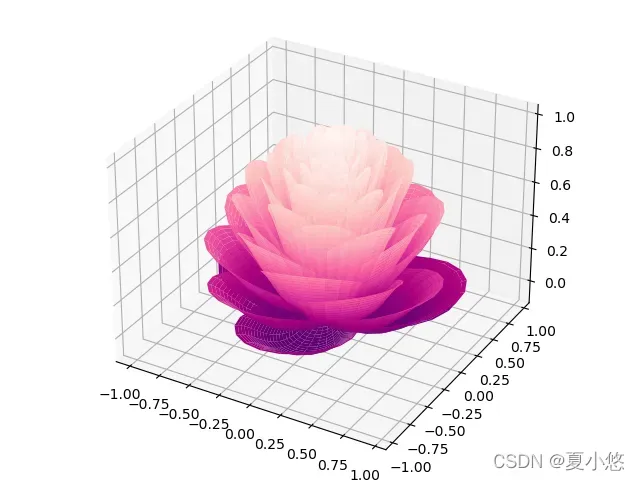
校正前后的图像差异如下：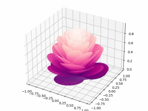

5. 结束语

3D花的绘制主要原理是极坐标，通过正弦/余弦函数进行旋转变形构造，参数略微变化就会出现不同的花朵，有趣！