0. 前言
在计算机视觉领域,轮廓通常指图像中对象边界的一系列点。因此,轮廓通常描述了对象边界的关键信息,包含了有关对象形状的主要信息,该信息可用于形状分析与对象检测和识别。我们已经在《OpenCV轮廓检测》中介绍了如何检测和绘制轮廓,在本文中,我们将继续学习如何利用获取到的轮廓,进行形状分析以及对象检测和识别。
1. 轮廓绘制
在《OpenCV轮廓检测》中,我们介绍了如何从图像矩计算获取轮廓属性(例如,质心,面积,圆度或偏心等)。除此之外,OpenCV还提供了一些其他用于进一步描述轮廓的函数。
cv2.boundingRect()返回包含轮廓所有点的最小边界矩形:
x, y, w, h = cv2.boundingRect(contours[0])
cv2.minAreaRect()返回包含轮廓所有点的最小旋转(如有必要)矩形:
rotated_rect = cv2.minAreaRect(contours[0])
为了提取旋转矩形的四个点,可以使用cv2.boxPoints()函数,返回旋转矩形的四个顶点:
box = cv2.boxPoints(rotated_rect)
cv2.minEnclosingCircle()返回包含轮廓所有点的最小圆(该函数返回圆心和半径):
(x, y), radius = cv2.minEnclosingCircle(contours[0])
cv2.fitEllipse()返回包含轮廓所有点的椭圆(具有最小平方误差):
ellipse = cv2.fitEllipse(contours[0])
cv2.approxPolyDP()基于给定精度返回给定轮廓的轮廓近似,此函数使用Douglas-Peucker算法:
approx = cv2.approxPolyDP(contours[0], epsilon, True)
其中,epsilon参数用于确定精度,确定原始曲线之间的最大距离及其近似。因此,由此产生的轮廓是类似于给定的轮廓的压缩轮廓。
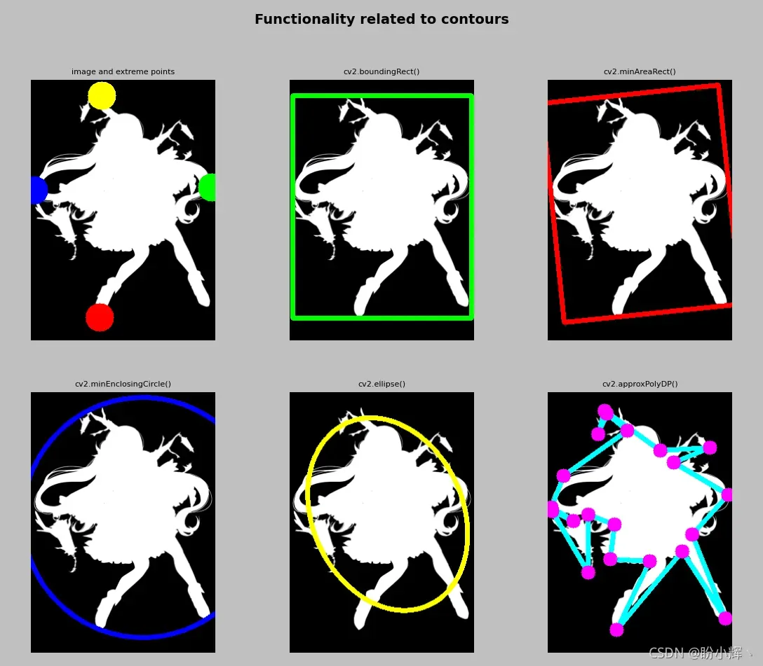
接下来,我们使用与轮廓相关的OpenCV函数计算给定轮廓的外端点,在具体讲解代码时,首先看下结果图像,以更好的理解上述函数:
首先编写extreme_points()用于计算定义给定轮廓的四个外端点:
def extreme_points(contour):
    """检测轮廓的极值点"""

    extreme_left = tuple(contour[contour[:, :, 0].argmin()][0])
    extreme_right = tuple(contour[contour[:, :, 0].argmax()][0])
    extreme_top = tuple(contour[contour[:, :, 1].argmin()][0])
    extreme_bottom = tuple(contour[contour[:, :, 1].argmax()][0])

    return extreme_left, extreme_right, extreme_top, extreme_bottom
np.argmin()沿轴返回最小值的索引,在多个出现最小值的情况下返回第一次出现的索引;而np.argmax()返回最大值的索引。一旦索引 index 计算完毕,就可以利用索引获取阵列的相应元素(例如,contour[index]——[[40 320]]),如果要访问第一个元素,则使用contour[index][0]——[40 320];最后,我们将其转换为元组:tuple(contour[index][0]——(40,320),用以绘制轮廓点。
def array_to_tuple(arr):
    """将列表转换为元组"""
    return tuple(arr.reshape(1, -1)[0])

def draw_contour_points(img, cnts, color):
    """绘制所有检测到的轮廓点"""
    for cnt in cnts:
        squeeze = np.squeeze(cnt)
        for p in squeeze:
            pp = array_to_tuple(p)
            cv2.circle(img, pp, 10, color, -1)
    return img

def draw_contour_outline(img, cnts, color, thickness=1):
    """绘制所有轮廓"""
    for cnt in cnts:
        cv2.drawContours(img, [cnt], 0, color, thickness)

def show_img_with_matplotlib(color_img, title, pos):
    """图像可视化"""
    img_RGB = color_img[:, :, ::-1]

    ax = plt.subplot(2, 3, pos)
    plt.imshow(img_RGB)
    plt.title(title, fontsize=8)
    plt.axis('off')

# 加载图像并转换为灰度图像
image = cv2.imread("example.png")
gray_image = cv2.cvtColor(image, cv2.COLOR_BGR2GRAY)

# 阈值处理转化为二值图像
ret, thresh = cv2.threshold(gray_image, 60, 255, cv2.THRESH_BINARY)

# 利用二值图像检测图像中的轮廓
contours, hierarchy = cv2.findContours(thresh, cv2.RETR_EXTERNAL, cv2.CHAIN_APPROX_NONE)

# 显示检测到的轮廓数
print("detected contours: '{}' ".format(len(contours)))
# 创建原始图像的副本以执行可视化
boundingRect_image = image.copy()
minAreaRect_image = image.copy()
fitEllipse_image = image.copy()
minEnclosingCircle_image = image.copy()
approxPolyDP_image = image.copy()

# 1. cv2.boundingRect()
x, y, w, h = cv2.boundingRect(contours[0])
cv2.rectangle(boundingRect_image, (x, y), (x + w, y + h), (0, 255, 0), 5)

# 2. cv2.minAreaRect()
rotated_rect = cv2.minAreaRect(contours[0])
box = cv2.boxPoints(rotated_rect)
box = np.int0(box)
cv2.polylines(minAreaRect_image, [box], True, (0, 0, 255), 5)

# 3. cv2.minEnclosingCircle()
(x, y), radius = cv2.minEnclosingCircle(contours[0])
center = (int(x), int(y))
radius = int(radius)
cv2.circle(minEnclosingCircle_image, center, radius, (255, 0, 0), 5)

# 4. cv2.fitEllipse()
ellipse = cv2.fitEllipse(contours[0])
cv2.ellipse(fitEllipse_image, ellipse, (0, 255, 255), 5)

# 5. cv2.approxPolyDP()
epsilon = 0.01 * cv2.arcLength(contours[0], True)
approx = cv2.approxPolyDP(contours[0], epsilon, True)
draw_contour_outline(approxPolyDP_image, [approx], (255, 255, 0), 5)
draw_contour_points(approxPolyDP_image, [approx], (255, 0, 255))

# 检测轮廓的极值点
left, right, top, bottom = extreme_points(contours[0])
cv2.circle(image, left, 20, (255, 0, 0), -1)
cv2.circle(image, right, 20, (0, 255, 0), -1)
cv2.circle(image, top, 20, (0, 255, 255), -1)
cv2.circle(image, bottom, 20, (0, 0, 255), -1)

# 可视化
show_img_with_matplotlib(image, "image and extreme points", 1)
show_img_with_matplotlib(boundingRect_image, "cv2.boundingRect()", 2)
show_img_with_matplotlib(minAreaRect_image, "cv2.minAreaRect()", 3)
show_img_with_matplotlib(minEnclosingCircle_image, "cv2.minEnclosingCircle()", 4)
show_img_with_matplotlib(fitEllipse_image, "cv2.ellipse()", 5)
show_img_with_matplotlib(approxPolyDP_image, "cv2.approxPolyDP()", 6)
plt.show()
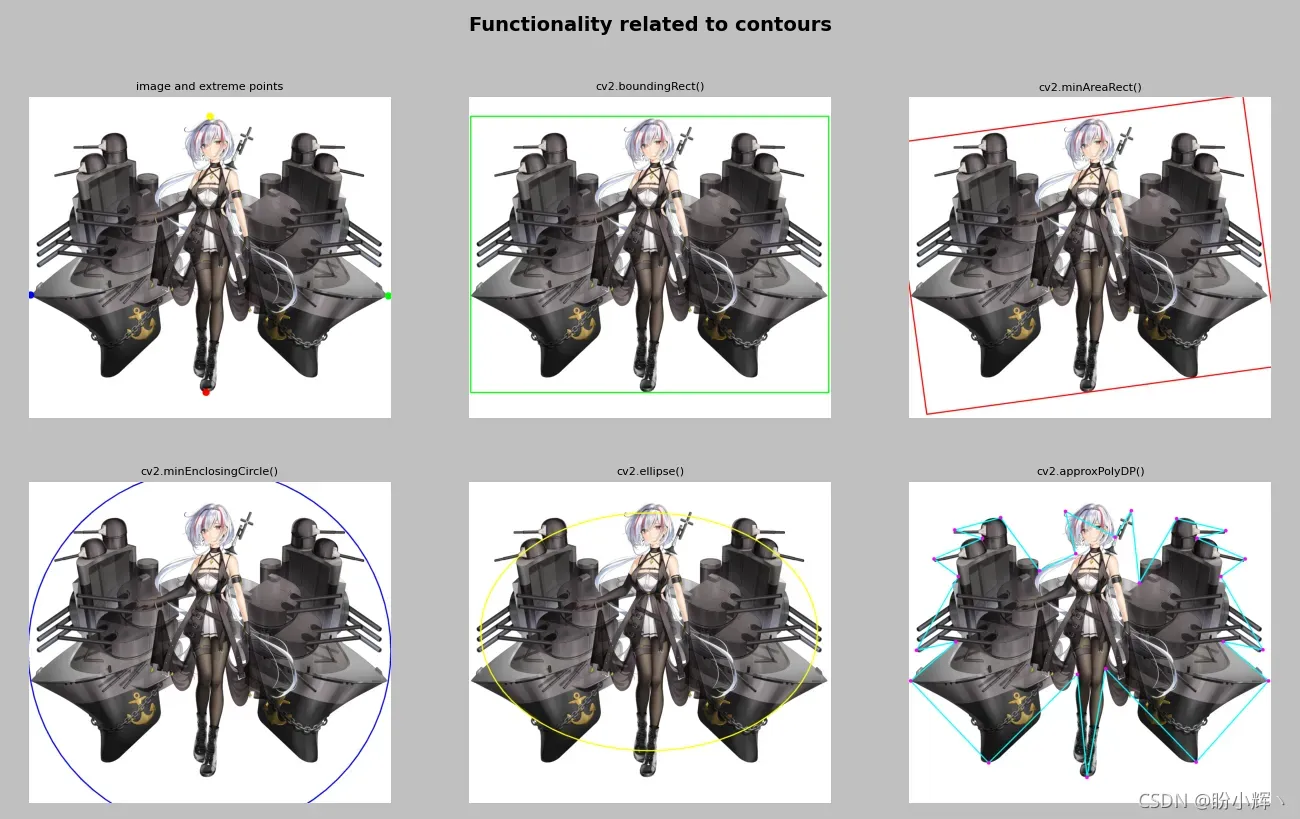
我们还可以在其他图像上测试效果:
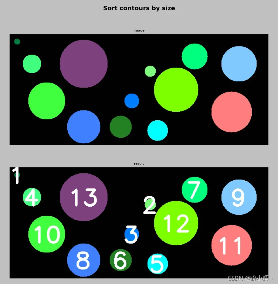
2. 轮廓筛选
如果想要计算检测到的轮廓的大小,可以使用基于图像矩的方法或使用OpenCV函数cv2.contourArea()来计算检测到的轮廓的大小,接下来,让我们将根据每个检测到的轮廓大小对其进行排序,在实践中,某些小的轮廓可能是噪声导致的,可能需要对轮廓进行筛选。
我们首先在画布上绘制不同半径的圆,以便后续检测:
# 画布
image = np.ones((300,700,3), dtype='uint8')
# 绘制不同半径的圆
cv2.circle(image, (20, 20), 8, (64, 128, 0), -1)
cv2.circle(image, (60, 80), 25, (128, 255, 64), -1)
cv2.circle(image, (100, 180), 50, (64, 255, 64), -1)
cv2.circle(image, (200, 250), 45, (255, 128, 64), -1)
cv2.circle(image, (300, 250), 30, (35, 128, 35), -1)
cv2.circle(image, (380, 100), 15, (125, 255, 125), -1)
cv2.circle(image, (600, 210), 55, (125, 125, 255), -1)
cv2.circle(image, (450, 150), 60, (0, 255, 125), -1)
cv2.circle(image, (330, 180), 20, (255, 125, 0), -1)
cv2.circle(image, (500, 60), 35, (125, 255, 0), -1)
cv2.circle(image, (200, 80), 65, (125, 64, 125), -1)
cv2.circle(image, (620, 80), 48, (255, 200, 128), -1)
cv2.circle(image, (400, 260), 28, (255, 255, 0), -1)
接下来,检测图中的轮廓:
gray_image = cv2.cvtColor(image, cv2.COLOR_BGR2GRAY)
# 阈值处理
ret, thresh = cv2.threshold(gray_image, 50, 255, cv2.THRESH_BINARY)
# 检测轮廓
contours, hierarchy = cv2.findContours(thresh, cv2.RETR_EXTERNAL, cv2.CHAIN_APPROX_NONE)
# 打印检测到的轮廓数
print("detected contours: '{}' ".format(len(contours)))
按每个检测到的轮廓的大小排序:
def sort_contours_size(cnts):
    """根据大小对轮廓进行排序"""

    cnts_sizes = [cv2.contourArea(contour) for contour in cnts]
    (cnts_sizes, cnts) = zip(*sorted(zip(cnts_sizes, cnts)))
    return cnts_sizes, cnts

(contour_sizes, contours) = sort_contours_size(contours)
最后用于可视化:
for i, (size, contour) in enumerate(zip(contour_sizes, contours)):
    # 计算轮廓的矩
    M = cv2.moments(contour)
    # 质心
    cX = int(M['m10'] / M['m00'])
    cY = int(M['m01'] / M['m00'])
    # get_position_to_draw() 函数与上例相同
    (x, y) = get_position_to_draw(str(i + 1), (cX, cY), cv2.FONT_HERSHEY_SIMPLEX, 2, 5)

    # 将排序结果置于形状的质心
    cv2.putText(image, str(i + 1), (x, y), cv2.FONT_HERSHEY_SIMPLEX, 2, (255, 255, 255), 5)
# show_img_with_matplotlib() 函数与上例相同
show_img_with_matplotlib(image, 'image', 1)
show_img_with_matplotlib(image, "result", 2)

plt.show()
运行程序的结果如下:
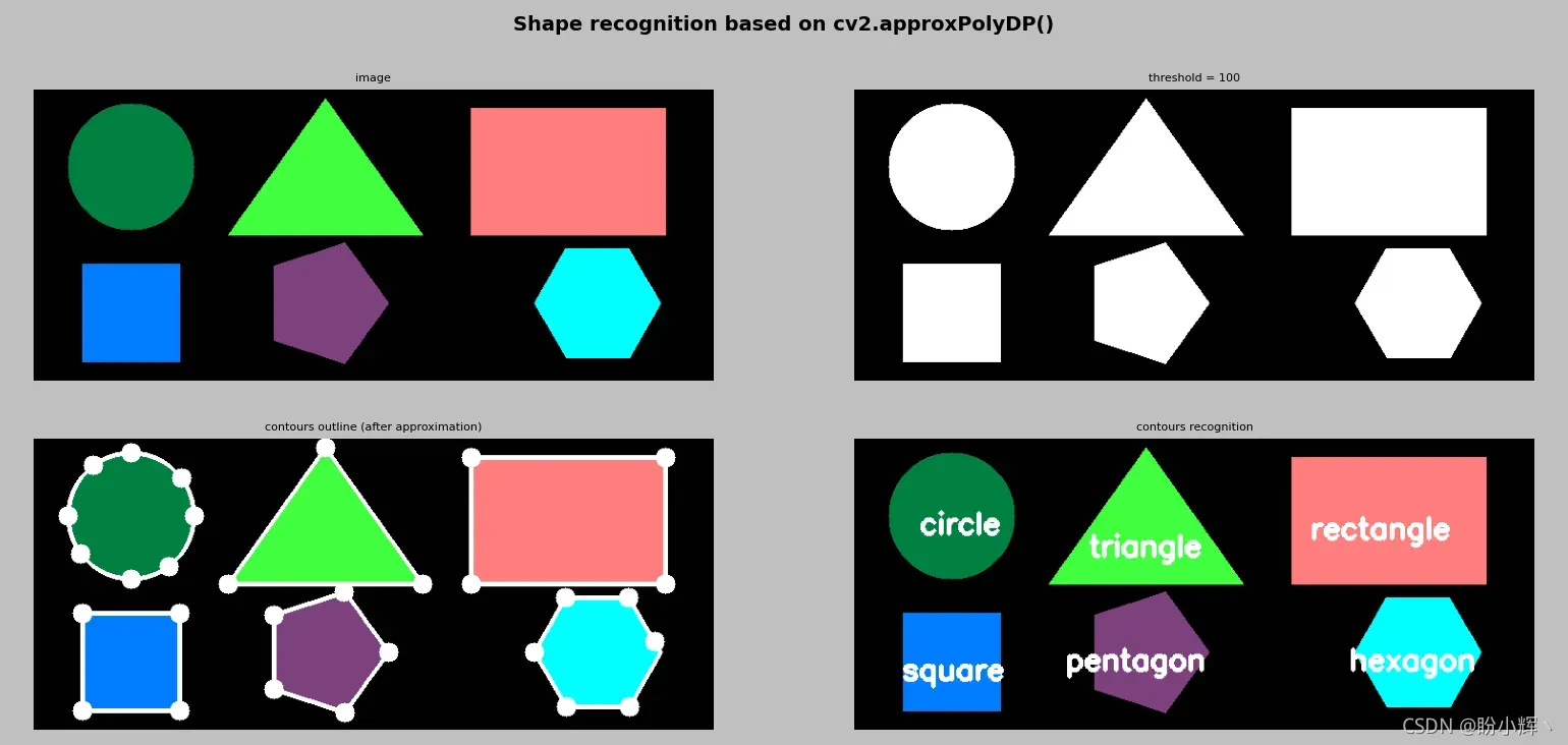
3. 轮廓识别
我们之前已经介绍了cv2.approxPolyDP(),它可以使用Douglas Peucker算法用较少的点来使一个轮廓逼近检测的轮廓。此函数中的一个关键参数是epsilon,其用于设置近似精度。我们使用cv2.approxPolyDP(),以便根据被抽取的轮廓中的检测到顶点的数量识别轮廓(例如,三角形,方形,矩形,五角形或六角形)。为了减少点数,给定某个轮廓,我们首先计算轮廓的边(perimeter)。基于边,建立epsilon参数,epsilon参数计算如下:
epsilon = 0.03 * perimeter
如果该常数变大(例如,从 0.03 变为 0.1 ),则epsilon参数也会更大,近似精度将减小,这导致具有较少点的轮廓,并且导致顶点的缺失,对轮廓的识别也将不正确,因为它基于检测到的顶点的数量;另一方面,如果该常数较小(例如,从0.03 变为 0.001),则epsilon参数也将变小,因此,近似精度将增加,将产生具有更多点的近似轮廓,对轮廓的识别同样会出现错误,因为获得了虚假顶点。
# 构建测试图像
image = np.ones((300,700,3), dtype='uint8')
cv2.circle(image, (100, 80), 65, (64, 128, 0), -1)
pts = np.array([[300, 10], [400, 150], [200, 150]], np.int32)
pts = pts.reshape((-1, 1, 2))
cv2.fillPoly(image, [pts], (64, 255, 64))
cv2.rectangle(image, (450, 20),(650, 150),(125, 125, 255),-1)
cv2.rectangle(image, (50, 180),(150, 280),(255, 125, 0),-1)
pts = np.array([[365, 220], [320, 282], [247, 258], [247, 182], [320, 158]], np.int32)
pts = pts.reshape((-1, 1, 2))
cv2.fillPoly(image, [pts], (125, 64, 125))
pts = np.array([[645, 220], [613, 276], [548, 276], [515, 220], [547, 164],[612, 164]], np.int32)
pts = pts.reshape((-1, 1, 2))
cv2.fillPoly(image, [pts], (255, 255, 0))

gray_image = cv2.cvtColor(image, cv2.COLOR_BGR2GRAY)

ret, thresh = cv2.threshold(gray_image, 50, 255, cv2.THRESH_BINARY)
# 轮廓检测
contours, hierarchy = cv2.findContours(thresh, cv2.RETR_EXTERNAL, cv2.CHAIN_APPROX_NONE)

image_contours = image.copy()
image_recognition_shapes = image.copy()

# 绘制所有检测的轮廓
draw_contour_outline(image_contours, contours, (255, 255, 255), 4)

def get_position_to_draw(text, point, font_face, font_scale, thickness):
    """获取图形坐标中心点"""
    text_size = cv2.getTextSize(text, font_face, font_scale, thickness)[0]
    text_x = point[0] - text_size[0] / 2
    text_y = point[1] + text_size[1] / 2
    return round(text_x), round(text_y)

def detect_shape(contour):
    """形状识别"""
    # 计算轮廓的周长
    perimeter = cv2.arcLength(contour, True)
    contour_approx = cv2.approxPolyDP(contour, 0.03 * perimeter, True)
    if len(contour_approx) == 3:
        detected_shape = 'triangle'
    elif len(contour_approx) == 4:
        x, y, width, height = cv2.boundingRect(contour_approx)
        aspect_ratio = float(width) / height
        if 0.90 < aspect_ratio < 1.10:
            detected_shape = "square"
        else:
            detected_shape = "rectangle"
    elif len(contour_approx) == 5:
        detected_shape = "pentagon"
    elif len(contour_approx) == 6:
        detected_shape = "hexagon"
    else:
        detected_shape = "circle"
    return detected_shape, contour_approx

for contour in contours:
    # 计算轮廓的矩
    M = cv2.moments(contour)
    # 计算轮廓的质心
    cX = int(M['m10'] / M['m00'])
    cY = int(M['m01'] / M['m00'])
    # 识别轮廓形状
    shape, vertices = detect_shape(contour)
    # 绘制轮廓
    draw_contour_points(image_contours, [vertices], (255, 255, 255))
    # 将形状的名称置于形状的质心
    (x, y) = get_position_to_draw(shape, (cX, cY), cv2.FONT_HERSHEY_SIMPLEX, 1.6, 3)
    cv2.putText(image_recognition_shapes, shape, (x+35, y), cv2.FONT_HERSHEY_SIMPLEX, 1, (255, 255, 255), 3)

# 可视化
show_img_with_matplotlib(image, "image", 1)
show_img_with_matplotlib(cv2.cvtColor(thresh, cv2.COLOR_GRAY2BGR), "threshold = 100", 2)
show_img_with_matplotlib(image_contours, "contours outline (after approximation)", 3)
show_img_with_matplotlib(image_recognition_shapes, "contours recognition", 4)
plt.show()
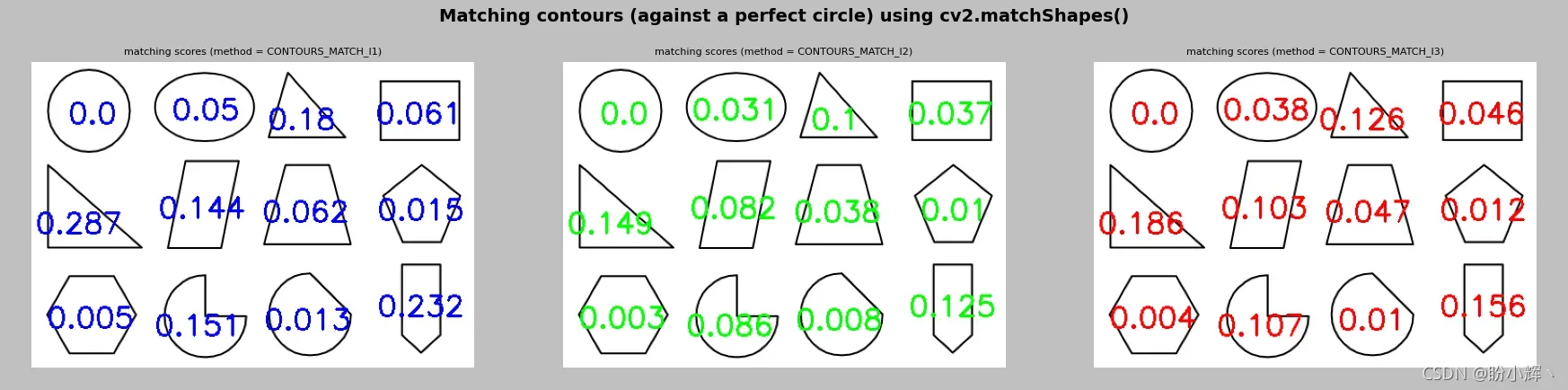
4. 轮廓匹配
Hu 矩不变性可用于对象匹配和识别,我们将介绍如何基于 Hu 矩不变性的匹配轮廓。OpenCV提供cv2.matchShapes()函数可用于比较两个轮廓,其包含三种匹配算法,包括cv2.CONTOURS_MATCH_I1,cv2.CONTOURS_MATCH_I2和cv2.CONTOURS_MATCH_I3,这些算法都使用Hu矩不变性。
如果 A 表示第一个对象,B 表示第二个对象,则使用以下公式计算匹配性:
其中,和
分别是 A 和 B 的 Hu 矩。
接下来,我们使用cv2.matchShapes()来计算轮廓与给定圆形轮廓的匹配程度。
首先,通过使用cv2.circle()在图像中绘制圆形作为参考图像。之后,加载绘制了不同形状的图像,然后在上述图像中查找轮廓:
def build_circle_image():
    """绘制参考圆"""
    img = np.zeros((500, 500, 3), dtype="uint8")
    cv2.circle(img, (250, 250), 200, (255, 255, 255), 1)
    return img
# 加载图像
image = cv2.imread("example.png")
gray_image = cv2.cvtColor(image, cv2.COLOR_BGR2GRAY)
image_circle = build_circle_image()
gray_image_circle = cv2.cvtColor(image_circle, cv2.COLOR_BGR2GRAY)

# 二值化图像
ret, thresh = cv2.threshold(gray_image, 70, 255, cv2.THRESH_BINARY_INV)
ret, thresh_circle = cv2.threshold(gray_image_circle, 70, 255, cv2.THRESH_BINARY)

# 检测轮廓
contours, hierarchy = cv2.findContours(thresh, cv2.RETR_EXTERNAL, cv2.CHAIN_APPROX_NONE)
contours_circle, hierarchy_2 = cv2.findContours(thresh_circle, cv2.RETR_EXTERNAL, cv2.CHAIN_APPROX_NONE)

result_1 = image.copy()
result_2 = image.copy()
result_3 = image.copy()

for contour in contours:
    # 计算轮廓的矩
    M = cv2.moments(contour)

    # 计算矩的质心
    cX = int(M['m10'] / M['m00'])
    cY = int(M['m01'] / M['m00'])

    # 使用三种匹配模式将每个轮廓与圆形轮廓进行匹配
    ret_1 = cv2.matchShapes(contours_circle[0], contour, cv2.CONTOURS_MATCH_I1, 0.0)
    ret_2 = cv2.matchShapes(contours_circle[0], contour, cv2.CONTOURS_MATCH_I2, 0.0)
    ret_3 = cv2.matchShapes(contours_circle[0], contour, cv2.CONTOURS_MATCH_I3, 0.0)

    # 将获得的分数写在结果图像中
    (x_1, y_1) = get_position_to_draw(str(round(ret_1, 3)), (cX, cY), cv2.FONT_HERSHEY_SIMPLEX, 1.2, 3)
    (x_2, y_2) = get_position_to_draw(str(round(ret_2, 3)), (cX, cY), cv2.FONT_HERSHEY_SIMPLEX, 1.2, 3)
    (x_3, y_3) = get_position_to_draw(str(round(ret_3, 3)), (cX, cY), cv2.FONT_HERSHEY_SIMPLEX, 1.2, 3)

    cv2.putText(result_1, str(round(ret_1, 3)), (x_1+10, y_1), cv2.FONT_HERSHEY_SIMPLEX, 1, (255, 0, 0), 2)
    cv2.putText(result_2, str(round(ret_2, 3)), (x_2+10, y_2), cv2.FONT_HERSHEY_SIMPLEX, 1, (0, 255, 0), 2)
    cv2.putText(result_3, str(round(ret_3, 3)), (x_3+10, y_3), cv2.FONT_HERSHEY_SIMPLEX, 1, (0, 0, 255), 2)
概括
在本文中,我们学习了如何利用获取到的轮廓,进行形状分析以及对象检测和识别,可以利用cv2.boundingRect()、cv2.minAreaRect()、cv2.minEnclosingCircle()、cv2.fillEllipse()和cv2.approxPolyDP()进行轮廓绘制,使用cv2.contourArea()计算轮廓面积,以及cv2.matchShapes()进行轮廓的匹配。
系列链接
OpenCV-Python实战(1)——OpenCV简介与图像处理基础
OpenCV-Python实战(2)——图像与视频文件的处理
OpenCV-Python实战(3)——OpenCV中绘制图形与文本
OpenCV-Python实战(4)——OpenCV常见图像处理技术
OpenCV-Python实战(5)——OpenCV图像运算
OpenCV-Python实战(6)——OpenCV中的色彩空间和色彩映射
OpenCV-Python实战(7)——直方图详解
OpenCV-Python实战(8)——直方图均衡化
OpenCV-Python实战(9)——OpenCV用于图像分割的阈值技术
OpenCV-Python实战(10)——OpenCV轮廓检测
OpenCV-Python实战(12)——一文详解AR增强现实
OpenCV-Python实战(13)——OpenCV与机器学习的碰撞
OpenCV-Python实战(14)——人脸检测详解
版权声明:本文为博主盼小辉丶原创文章,版权归属原作者,如果侵权,请联系我们删除!
原文链接:https://blog.csdn.net/LOVEmy134611/article/details/120899474