(一)tensors
张量是一种特殊的数据结构,与数组矩阵类似,在pytoch中,使用tensors对模型的输入和输出进行编码
import torch
import numpy as np
1.tensor 初始化
# 直接数据
data=[[1,2],[3,4]]
x_data=torch.tensor(data)
# numpy 数组
np_array=np.array(data)
x_np=torch.from_numpy(np_array)
# 从另一个tensor
x_ones=torch.ones_like(x_data)#保留shape,datatype
print(f'ones tensor:\n{x_ones}\n')
x_rands=torch.rand_like(x_data,dtype=torch.float)#保留shape
print(f'random tensor:\n{x_rands}\n')
ones tensor:
tensor([[1, 1],
        [1, 1]])

random tensor:
tensor([[0.3272, 0.3049],
        [0.3315, 0.8603]])
shape是tensor维度
shape=(2,3,)
rand_tensor=torch.rand(shape)
ones_tensor=torch.ones(shape)
zeros_tensor=torch.zeros(shape)
print(rand_tensor)
print(ones_tensor)
print(zeros_tensor)
tensor([[0.3955, 0.7930, 0.1733],
        [0.3849, 0.5444, 0.3754]])
tensor([[1., 1., 1.],
        [1., 1., 1.]])
tensor([[0., 0., 0.],
        [0., 0., 0.]])
2.tensor 性质
shape,datatype,device(存储位置)
tensor=torch.rand(3,4)
print(tensor.shape,'\n',tensor.dtype,'\n',tensor.device)
torch.Size([3, 4])
 torch.float32
 cpu
3.tensor 运算
转置、索引、切片、数学、线性代数、随机采样
# 索引和切片
tensor=torch.ones(4,4)
tensor[:,1]=0
print(tensor)
tensor([[1., 0., 1., 1.],
        [1., 0., 1., 1.],
        [1., 0., 1., 1.],
        [1., 0., 1., 1.]])
# 连接
t1=torch.cat([tensor,tensor,tensor],dim=1)
t1
tensor([[1., 0., 1., 1., 1., 0., 1., 1., 1., 0., 1., 1.],
        [1., 0., 1., 1., 1., 0., 1., 1., 1., 0., 1., 1.],
        [1., 0., 1., 1., 1., 0., 1., 1., 1., 0., 1., 1.],
        [1., 0., 1., 1., 1., 0., 1., 1., 1., 0., 1., 1.]])
# 数字乘
tensor.mul(tensor)
tensor*tensor
# 矩阵乘
tensor.matmul(tensor.T)
tensor@tensor.T
tensor([[3., 3., 3., 3.],
        [3., 3., 3., 3.],
        [3., 3., 3., 3.],
        [3., 3., 3., 3.]])
# 就地操作_
print(tensor)
tensor.add_(4)
print(tensor)
tensor([[1., 0., 1., 1.],
        [1., 0., 1., 1.],
        [1., 0., 1., 1.],
        [1., 0., 1., 1.]])
tensor([[5., 4., 5., 5.],
        [5., 4., 5., 5.],
        [5., 4., 5., 5.],
        [5., 4., 5., 5.]])
4.bridge numpy
# tensor-->numpy
t=torch.ones(5)
print(f't:{t}')
n=t.numpy()
print(f'n:{n}')
t:tensor([1., 1., 1., 1., 1.])
n:[1. 1. 1. 1. 1.]
# tensor变化会在numpy中反应
t.add_(1)
print(t)
print(n)
tensor([2., 2., 2., 2., 2.])
[2. 2. 2. 2. 2.]
# numpy-->tensor
n=np.ones(5)
t=torch.from_numpy(n)
np.add(n,1,out=n)
print(t)
print(n)
tensor([2., 2., 2., 2., 2.], dtype=torch.float64)
[2. 2. 2. 2. 2.]
(二)torch.autograd
pytorch自动差分引擎,可为神经网络训练提供支持
1.usage in pytorch
import ssl
ssl._create_default_https_context = ssl._create_unverified_context
import torch,torchvision
model=torchvision.models.resnet18(pretrained=True)
data=torch.rand(1,3,64,64)
labels=torch.rand(1,1000)
prediction=model(data)#forward
loss=(prediction-labels).sum()#loss function
loss.backward()#backward
optim=torch.optim.SGD(model.parameters(),lr=1e-2,momentum=0.9)#lr学习率
optim.step()#初始化梯度下降
2.differentiation in autograd
import torch
#requires_grad=True:every operation on them should be tracked.
a=torch.tensor([2.,3.],requires_grad=True)
b=torch.tensor([6.,4.],requires_grad=True)
#a,b是NN参数,Q是误差
Q=3*a**3-b**2
external_grad=torch.tensor([1,1])
#Q.backward:计算Q对a,b的gradients并储存在tensor.grad中
Q.backward(gradient=external_grad)
print(a.grad)
print(b.grad)
tensor([36., 81.])
tensor([-12.,  -8.])
3.computational graph
autograd保留DAG(有向无环图,包含函数对象)中的所有数据(tensors)和操作
1.前向传播:计算结果tensor,记录gradient function(leaves–root)
2.反向传播:计算每个参数的梯度并保存在tensor.grad中,链式法则(root–leaves)
x=torch.rand(5,5)
y=torch.rand(5,5)
z=torch.rand((5,5),requires_grad=True)
a=x+y
print(a.requires_grad)
b=x+z
print(b.requires_grad)
False
True
frozen parameters:不计算梯度的参数,减少计算量
from torch import nn,optim
model=torchvision.models.resnet18(pretrained=True)
#frozen 所有的参数除了function的权重和偏差
for param in model.parameters():
    param.requires_grad=False
model.fc=nn.Linear(512,10)
optimizer=optim.SGD(model.parameters(),lr=1e-2, momentum=0.9)
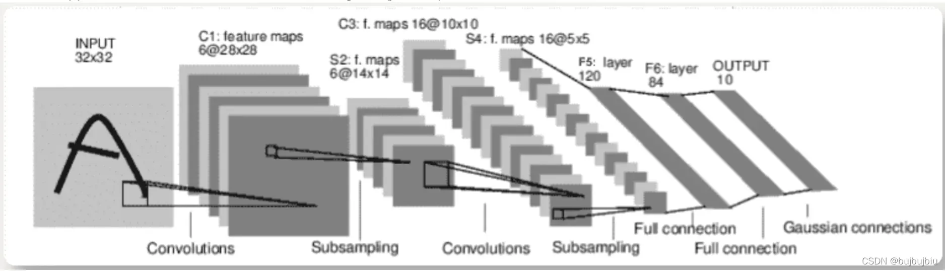
(3) 神经网络
torch.nn包构建神经网络
神经网络训练步骤:
1.定义神经网络(包含一些需要学习的参数/权重)
2.遍历输入数据集
3.通过网络处理输入
4.计算损失函数
5.网络参数梯度反向传播
6.通常使用简单的更新规则来更新网络的权重:weight = weight – learning_rate * gradient
1.define network
(1)Containers:
- Module:所有神经网络模型的基类
(2)Convolution Layers:
- nn.Conv2d:Applies a 2D convolution over an input signal composed of several input planes
(3)Linear Layers
- nn.Linear:Applies a linear transformation to the incoming data(y=wx+b)
import torch
import torch.nn as nn
import torch.nn.functional as F
class Net(nn.Module):

    def __init__(self):
        super(Net, self).__init__()
        # 1 input image channel, 6 output channels, 5x5 square convolution
        # kernel
        self.conv1 = nn.Conv2d(1, 6, 5)
        self.conv2 = nn.Conv2d(6, 16, 5)
        # an affine operation: y = Wx + b
        self.fc1 = nn.Linear(16 * 5 * 5, 120)  # 5*5 from image dimension
        self.fc2 = nn.Linear(120, 84)
        self.fc3 = nn.Linear(84, 10)

    def forward(self, x):
        # Max pooling over a (2, 2) window
        x = F.max_pool2d(F.relu(self.conv1(x)), (2, 2))
        # If the size is a square, you can specify with a single number
        x = F.max_pool2d(F.relu(self.conv2(x)), 2)
        x = torch.flatten(x, 1) # flatten all dimensions except the batch dimension
        x = F.relu(self.fc1(x))
        x = F.relu(self.fc2(x))
        x = self.fc3(x)
        return x
net = Net()
print(net)
Net(
  (conv1): Conv2d(1, 6, kernel_size=(5, 5), stride=(1, 1))
  (conv2): Conv2d(6, 16, kernel_size=(5, 5), stride=(1, 1))
  (fc1): Linear(in_features=400, out_features=120, bias=True)
  (fc2): Linear(in_features=120, out_features=84, bias=True)
  (fc3): Linear(in_features=84, out_features=10, bias=True)
)
只需要定义forward函数,就可以使用autograd自定义backward函数
模型学习参数由net.parameters()返回
params = list(net.parameters())
print(len(params))
print(params[0].size())#卷积层1的权重
#print(params)
10
torch.Size([6, 1, 5, 5])
input = torch.randn(1,1,32,32)
out = net(input)
print(out)
tensor([[ 0.0735, -0.0377,  0.1258, -0.0828, -0.0173, -0.0726, -0.0875, -0.0256,
         -0.0797,  0.0959]], grad_fn=<AddmmBackward0>)
使用随机梯度将所有参数和梯度缓冲区归零以进行反向传播
net.zero_grad
out.backward(torch.randn(1,10))
torch.nn仅支持小批量。 整个torch.nn包仅支持作为微型样本而不是单个样本的输入。例如,nn.Conv2d采用nSamples x nChannels x Height x Width的4D张量
目前看到的课程:
- torch.Tensor:一个多维数组,支持backward()的自动微分操作,保存张量梯度
- nn.Module:神经网络模块,封装参数
- nn.Parameter:一种张量,将其分配为Module的属性时,自动注册为参数
- autograd.Function:实现自动微分操作的正向和反向定义,每个Tensor操作都会创建至少一个Function节点,该节点连接到创建Tensor的函数,并且编码其历史记录。
2.loss function
损失函数采用(输出,目标)作为输入,并计算一个值估计输出与目标之间的距离,nn包有好几种不同的损失函数,简单的如nn.MSELoss,计算均方误差
output = net(input)
target = torch.randn(10)#只是用于例子
target = target.view(1,-1)#使其与输出保持相同shape
criterion = nn.MSELoss()
loss = criterion(output,target)
print(loss)
tensor(0.4356, grad_fn=<MseLossBackward0>)
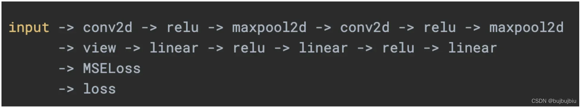
使用.grad_fn属性向后跟随loss,将得到一个计算图,调用loss.backward()时,整个图被微分,图中具有requires_grad=True的所有张量将随梯度累积其.grad张量
print(loss.grad_fn) # MSELoss
print(loss.grad_fn.next_functions[0][0]) # linear
print(loss.grad_fn.next_functions[0][0].next_functions[0][0]) # relu
<MseLossBackward0 object at 0x7fef4965df10>
<AddmmBackward0 object at 0x7fef4965d3a0>
<AccumulateGrad object at 0x7fef4965df10>
3.Backprop
反向传播,只需要loss.backward(),在此之前先清除现有梯度,否则梯度将累计到现在的梯度中
net.zero_grad() # 清除梯度

print('conv1的前偏差梯度')
print(net.conv1.bias.grad)

loss.backward()

print('conv1的后偏差梯度')
print(net.conv1.bias.grad)
conv1的前偏差梯度
tensor([0., 0., 0., 0., 0., 0.])
conv1的后偏差梯度
tensor([ 0.0124,  0.0051, -0.0029, -0.0088,  0.0048,  0.0012])
4.Update the weights
最简单的更新规则是随机梯度下降(SGD)
- weight = weight – learning_rate * gradient
learning_rate = 0.01
for f in net.parameters():
    f.data.sub_(f.grad.data*learning_rate)
但是使用神经网络时,可能需要用到不用的更新规则,如SGD,Nesterov-SGD,Adam,RMSProp等,使用torch.optim包可实现所有方法
import torch.optim as optim

# 创建optimizer
optimizer = optim.SGD(net.parameters(),lr=0.01)

# 在training loop里
optimizer.zero_grad() # 将梯度缓冲区手动设置为0
output = net(input)
loss = criterion(output,target)
loss.backward()
optimizer.step()
print(net.conv1.bias.grad)
tensor([ 0.0119, 0.0050, -0.0034, -0.0109, 0.0049, -0.0009])
版权声明:本文为博主bujbujbiu原创文章,版权归属原作者,如果侵权,请联系我们删除!
原文链接:https://blog.csdn.net/weixin_45526117/article/details/123009192