本文章包含以下内容:
1、灰度阀值分割
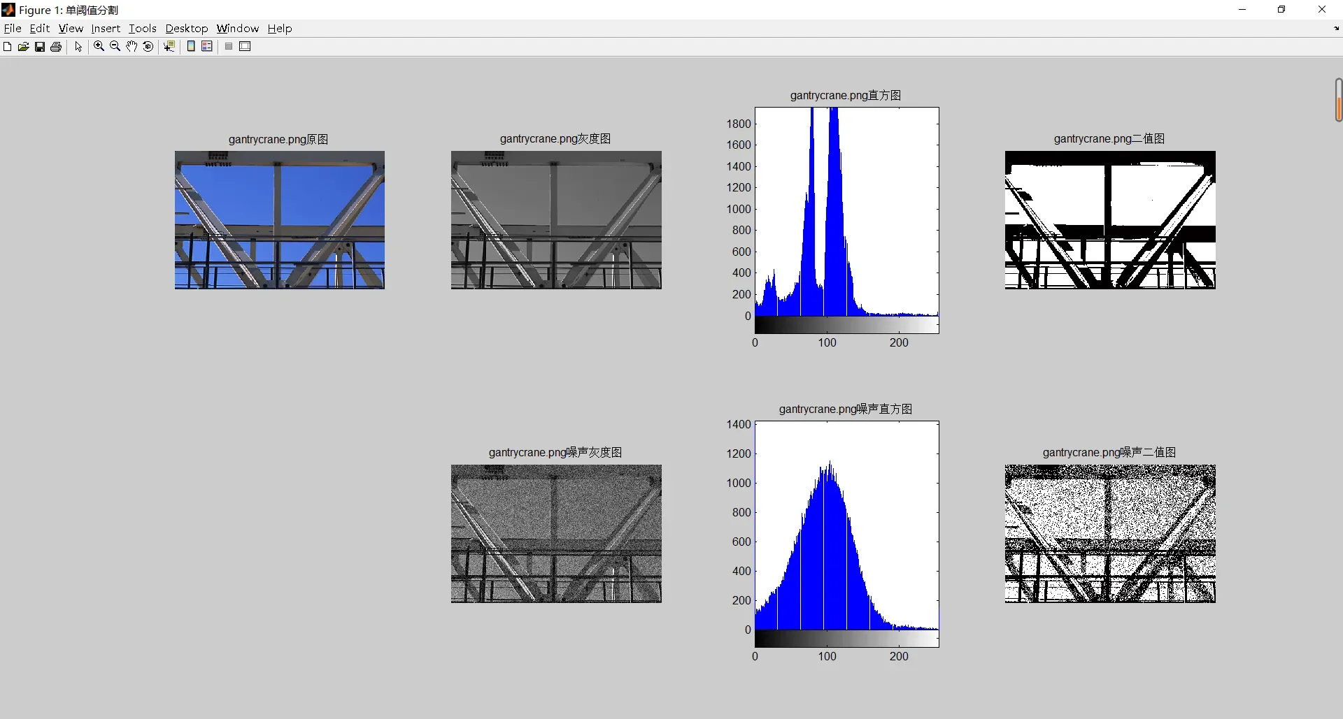
(1)单阈值分割图像
先将一幅彩色图像转换为灰度图像,显示其直方图,参考直方图中灰度的分布,尝试确定阈值;应反复调节阈值的大小,直至二值化的效果最为满意为止。给图像加上零均值的高斯噪声重复上述过程,注意阈值的选择。
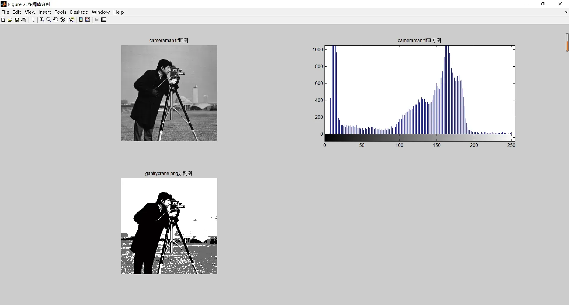
(2)多阈值分割图像
自选图像,对图进行多阈值分割,注意阈值的选择。
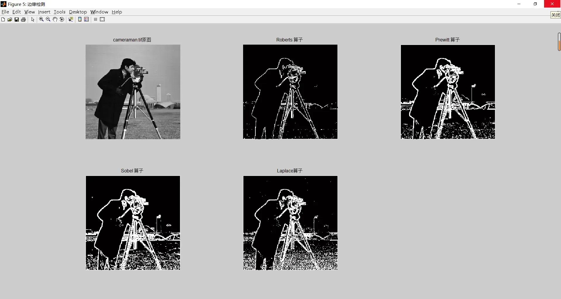
2.边缘检测
(1)使用Roberts 算子的图像分割实验,调入并显示一幅图像*.gif或*.tif;
使用Roberts 算子对图像进行边缘检测处理;Roberts 算子为一对模板,相应的矩阵为:
rh = [0 1;-1 0]; rv = [1 0;0 -1];
这里的rh 为水平Roberts 算子,rv为垂直Roberts 算子。可以显示处理后
的水平边界和垂直边界检测结果;
用“欧几里德距离”方式计算梯度的模,显示检测结果;对于检测结果进行二值化处理,并显示处理结果。
(2)使用Prewitt 算子的图像分割实验使用Prewitt 算子进行内容(1)中的全部步骤。
(3)使用Sobel 算子的图像分割实验使用Sobel 算子进行内容(1)中的全部步骤。
(4)使用Canny算子进行图像分割实验。
(5) 使用拉普拉斯算子进行图像分割实验。
代码如下:
function U()
    clear;
    clc;
    Single_threshold_segmentation()
    Multi_threshold_segmentation()
    edge_detection()
end

% 单阈值分割
% 先将一幅彩色图像转换为灰度图像,显示其直方图,
% 参考直方图中灰度的分布,尝试确定阈值
% 给图像加上零均值的高斯噪声重复上述过程
function Single_threshold_segmentation()
    img = imread('gantrycrane.png');    % 读取图像
    figure('Name','单阈值分割');  % 开一个叫单阈值分割的窗口
    subplot(2,4,1);imshow(img);title('gantrycrane.png原图');   % 显示原图
    img = rgb2gray(img);    % 彩色图像转为灰度图像
    subplot(2,4,2);imshow(img);title('gantrycrane.png灰度图');   % 显示灰度图
    subplot(2,4,3);imhist(img);title('gantrycrane.png直方图');   % 显示直方图
    % x = 95; % 分割阈值
    % img1 = uint8((0*(img<=x)+255.*(img>x))); % 图像分割
    x = graythresh(img);    % 分割阈值
    img1 = im2bw(img,x);    % 图像分割
    subplot(2,4,4);imshow(img1);title('gantrycrane.png二值图');   % 显示二值图
    img = imnoise(img,'gaussian');        % 添加高斯噪声
    subplot(2,4,6);imshow(img);title('gantrycrane.png噪声灰度图');   % 显示噪声灰度图
    subplot(2,4,7);imhist(img);title('gantrycrane.png噪声直方图');   % 显示噪声直方图
    % x = 95; % 分割阈值
    % img1 = uint8((0*(img<=x)+255.*(img>x))); % 图像分割
    x = graythresh(img);    % 分割阈值
    img1 = im2bw(img,x);    % 图像分割
    subplot(2,4,8);imshow(img1);title('gantrycrane.png噪声二值图');   % 显示噪声二值图
end
% 多阈值分割
function Multi_threshold_segmentation()
    img = imread('cameraman.tif');    % 读取图像
    figure('Name','多阈值分割');  % 开一个叫多阈值分割的窗口
    subplot(2,2,1);imshow(img);title('cameraman.tif原图');   % 显示原图
    subplot(2,2,2);imhist(img);title('cameraman.tif直方图');   % 显示直方图
    x_1 = 77; % 分割阈值
    x_2 = 139;
    img1 = uint8(0*(img<=x_1)+round((x_1+x_2)/2)*((img>x_1)&(img<=x_2))+255*(img>x_2)); % 图像分割
    subplot(2,2,3);imshow(img1);title('gantrycrane.png分割图');   % 显示分割图
end

% 边缘检测
% 使用Roberts,Prewitt,Sobel,Canny,拉普拉斯算子
function edge_detection()
    img = imread('cameraman.tif');  % 读取图像
    figure('Name','边缘检测');  % 开一个叫边缘检测的窗口
    subplot(2,3,1);imshow(img);title('cameraman.tif原图');   % 显示原图
    img1 = ed(img,[[0 1;-1 0];[1 0;0 -1]]);    % 使用 Roberts 算子
    subplot(2,3,2);imshow(img1);title('Roberts 算子');   % Roberts 算子处理图像
    img1 = ed(img,[[-1 -1 -1;0 0 0;1 1 1];[-1 0 1;-1 0 1;-1 0 1]]);    % 使用 Prewitt 算子
    subplot(2,3,3);imshow(img1);title('Prewitt 算子');   % Prewitt 算子处理图像
    img1 = ed(img,[[-1 -2 -1;0 0 0;1 2 1];[-1 0 1;-2 0 2;-1 0 1;]]);    % 使用 Sobel 算子
    subplot(2,3,4);imshow(img1);title('Sobel 算子');   % Sobel 算子处理图像
    img1 = ed(img,[[-1 1;-1 1];[-1 -1;1 1]]);    % 使用 Canny算子
    subplot(2,3,5);imshow(img1);title('Canny算子');   % Canny算子处理图像
    img1 = ed(img,[[0 -1 0;-1 4 -1;0 -1 0];[-1 -1 -1;-1 8 -1;-1 -1 -1]]);    % 使用 Laplace算子
    subplot(2,3,5);imshow(img1);title('Laplace算子');   % Laplace算子处理图像
end

% 进行卷积和二值化
function img2 = ed(img,x)
    s = size(x);
    img1 = zeros(size(img));
    for i = 1:s(1)/s(2)
        img1 = img1 + abs(conv2(img,x(1+s(2)*(i-1):s(2)*i,1:s(2)),'same'));
    end
    img1 = uint8(img1);
    img2 = im2bw(img1,graythresh(img1));
end
结果如下:
文章出处登录后可见!
已经登录?立即刷新