1 Pytorch模型转Onnx

对ONNX的介绍强烈建议看，本文做了很多参考：模型部署入门教程（一）：模型部署简介
 模型部署入门教程（三）：PyTorch 转 ONNX 详解
以及Pytorch的官方介绍：(OPTIONAL) EXPORTING A MODEL FROM PYTORCH TO ONNX AND RUNNING IT USING ONNX RUNTIME
C++的部署：详细介绍 Yolov5 转 ONNX模型 + 使用 ONNX Runtime 的 C++ 部署（包含官方文档的介绍）。

1.1 获得自己的PyTorch模型

我用的是自己训练好的一个yolov5-5.0模型。

1.2 Yolov5-5.0 的模型转换成 ONNX 格式的模型

PyCharm环境如下:
在这里插入图片描述
yolov5 可以使用官方的 export.py 脚本进行转换，这里不做详细解析
可参考：yolov5转onnx，c++调用完美复现
在网站 Netron （开源的模型可视化工具）来可视化 ONNX 模型。
想要理解 1.2 节的内容，请看对参数详细介绍的第3章。

1.2.1 查看导出的模型（多输出版本）

点击input 或者 output，可以查看 ONNX 模型的基本信息，包括模型的版本信息，以及模型输入、输出的名称和数据类型。参数具体代表什么看第3章。。
此处三个输出的 onnx 模型只是为了便于只管的看出参数的维度，实际上部署的话使用单输出的onnx模型，单输出的模型见下面的第二张图的部分。
如果导出为动态：python ./models/export.py --weights ./weights/best20221027.pt --img 640 --batch 1 --dynamic

1.2.2 查看导出的模型（单输出版本）

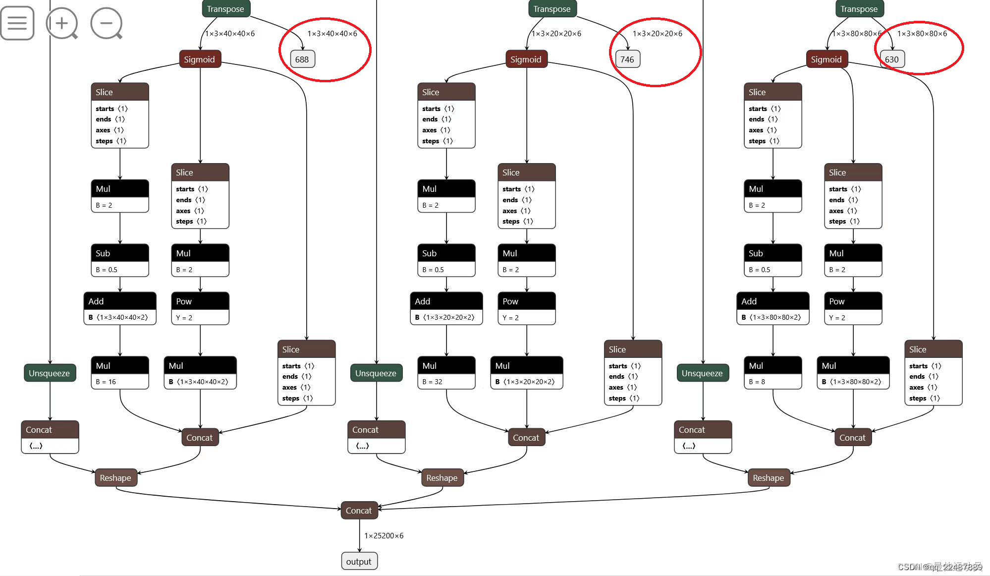
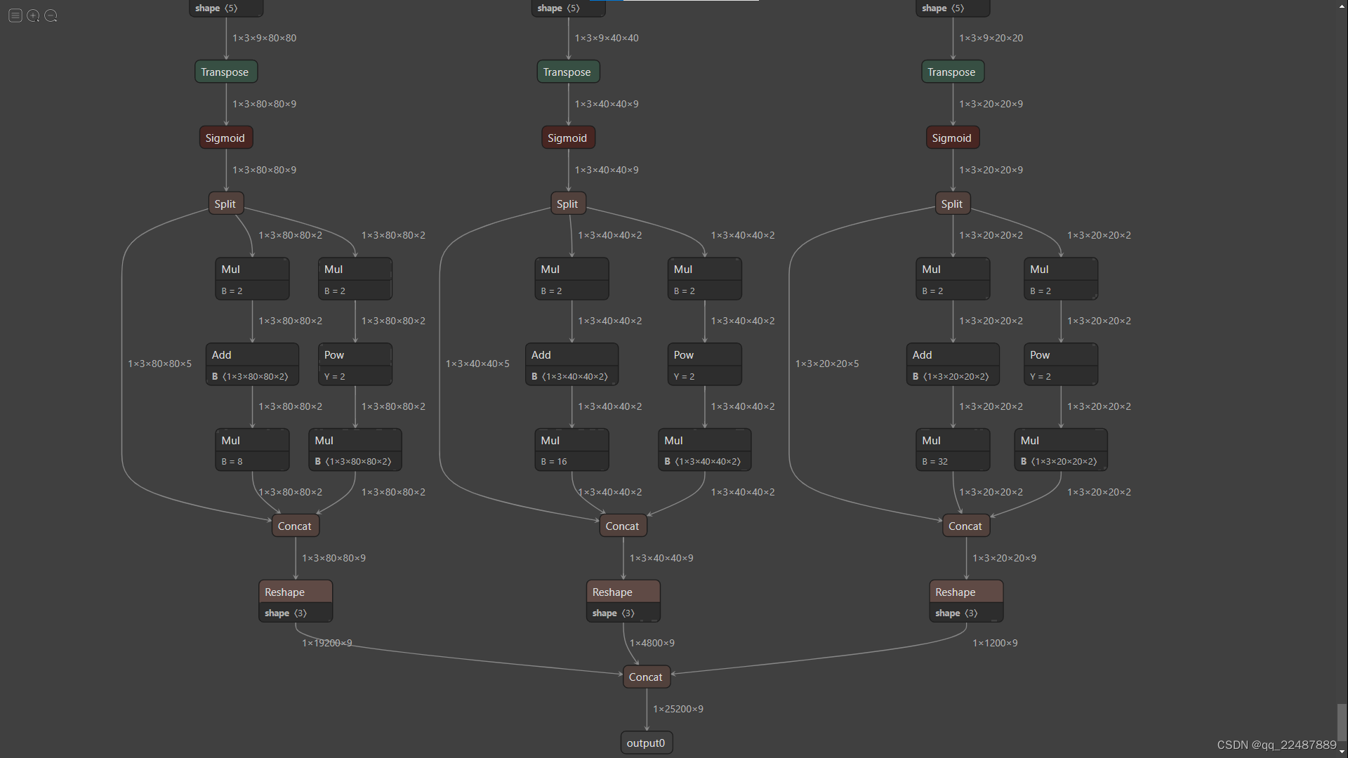
上面的三个输出结构很清晰，但是这种多输出的情况是一个问题，维度太多且参数还没有进行处理，很很很不利于部署，不如在导出的时候就处理好参数为单输出的情况，输出转成常用的 1 × Anchors数目 × 9（即红圈中的结果转换成），这样的话每个Anchor的坐标信息就是映射到原图中的，省去了很多处理数据的麻烦。步骤如下，参考 YOLOv5导出onnx、TrensorRT部署（LINUX）：

我采取的方案是，训练好的模型用yolov5-master的export.py来导出即可解决：python ./export.py --weights ./best20221027.pt --img 640 --batch 1 --include=onnx
得到的onnx文件如下！ 25200 = 3 × ( 80² + 40² + 20² ），接下来就可以部署了

onnx模型可视化，看出输出部分进行的处理如下：三输出模型的输出结果是 t_x t_y t_w t_h 和 t₀，即下图中sigmoid之前的参数，单输出的模型直接输出的是 b_x b_y b_w b_h 和 score，即直接对应到原图中的坐标参数。

如果此时导出为动态模型python ./export.py --weights ./best20221027.pt --img 640 --batch 1 --dynamic ，则如下图所示：
点击某一个算子节点，可以看到算子的具体信息。比如点击第一个 Conv 可以看到每个算子记录了算子属性、图结构、权重三类信息。

1.3 简化 ONNX 模型

参考：【OpenVino CPU模型加速（二）】使用openvino加速推理
 yolov5部署1——pytorch-＞onnx
简化步骤：

pip install onnx-simplifier
python -m onnxsim input_onnx_model output_onnx_model

结果如下：

python -m onnxsim  ./best20221027.onnx ./sim_best20221027.onnx

Simplifying...
Finish! Here is the difference:
┏━━━━━━━━━━━━┳━━━━━━━━━━━━━━━━┳━━━━━━━━━━━━━━━━━━┓
┃            ┃ Original Model ┃ Simplified Model ┃
┡━━━━━━━━━━━━╇━━━━━━━━━━━━━━━━╇━━━━━━━━━━━━━━━━━━┩
│ Add        │ 7              │ 7                │
│ Concat     │ 14             │ 14               │
│ Constant   │ 34             │ 0                │
│ Conv       │ 62             │ 62               │
│ MaxPool    │ 3              │ 3                │
│ Mul        │ 59             │ 59               │
│ Reshape    │ 3              │ 3                │
│ Resize     │ 2              │ 2                │
│ Sigmoid    │ 59             │ 59               │
│ Slice      │ 8              │ 8                │
│ Transpose  │ 3              │ 3                │
│ Model Size │ 27.0MiB        │ 27.0MiB          │
└────────────┴────────────────┴──────────────────┘

Constant 变成了 0 ，得到了简化。

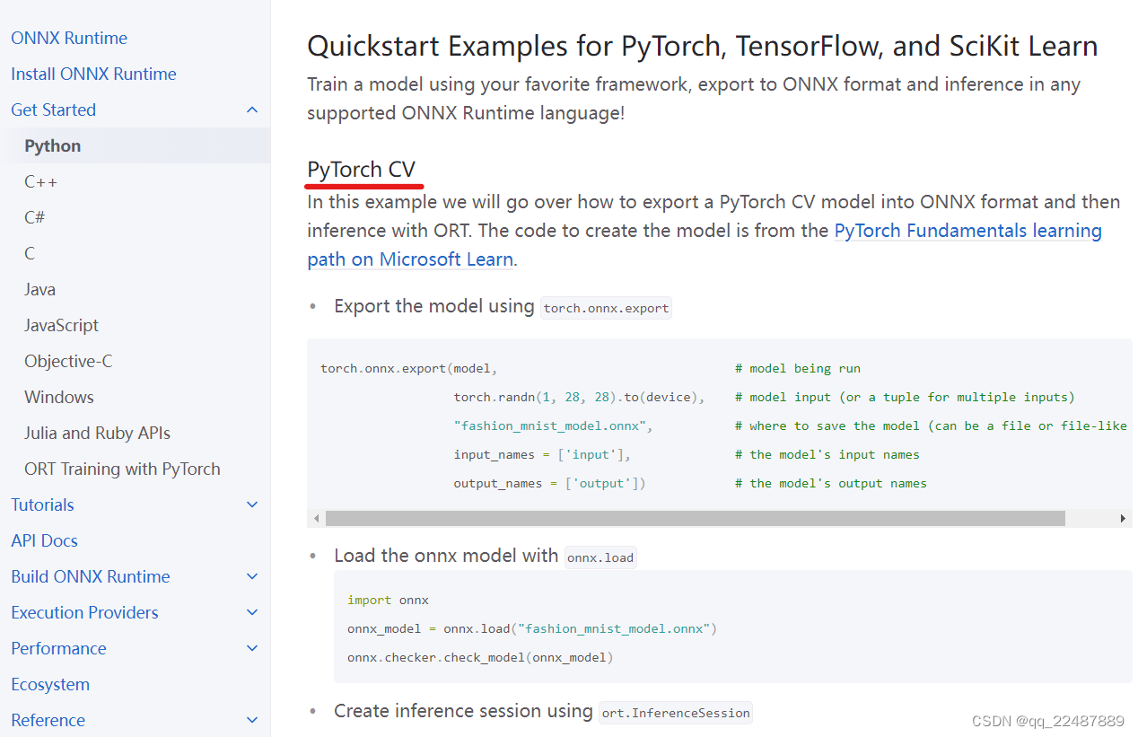
2 ONNX Runtime（Python）读取并运行 ONNX 格式的模型

onnxruntime python 推理模型，主要是为了测试模型的准确，模型部署的最终目的的用 C++ 部署，从而部署在嵌入式设备等。
ONNX Runtime Docs（官方文档）
推理总流程示例如下：

# 检验模型是否正确
import onnx
onnx_model = onnx.load("fashion_mnist_model.onnx")
onnx.checker.check_model(onnx_model)

# 加载和运行 ONNX 模型，以及指定环境和应用程序配置
import onnxruntime as ort
import numpy as np
x, y = test_data[0][0], test_data[0][1]
ort_sess = ort.InferenceSession('fashion_mnist_model.onnx')
outputs = ort_sess.run(None, {'input': x.numpy()})

# Print Result 
predicted, actual = classes[outputs[0][0].argmax(0)], classes[y]
print(f'Predicted: "{predicted}", Actual: "{actual}"')

推理的全部代码如下：其中 输入和输出的数据 需要根据ONNX模型的输入输出格式进行处理
代码参考的文章是（基本是复制过来进行微小修改和添加注释，建议收藏原文）：YOLOV5模型转onnx并推理，后面的章节均是对代码的介绍。

import onnx
import onnxruntime as ort
import numpy as np

import sys

import onnx
import onnxruntime as ort
import cv2
import numpy as np

CLASSES = ['person', 'bicycle', 'car', 'motorcycle', 'airplane', 'bus', 'train', 'truck', 'boat', 'traffic light',
           'fire hydrant', 'stop sign', 'parking meter', 'bench', 'bird', 'cat', 'dog', 'horse', 'sheep', 'cow',
           'elephant', 'bear', 'zebra', 'giraffe', 'backpack', 'umbrella', 'handbag', 'tie', 'suitcase', 'frisbee',
           'skis', 'snowboard', 'sports ball', 'kite', 'baseball bat', 'baseball glove', 'skateboard', 'surfboard',
           'tennis racket', 'bottle', 'wine glass', 'cup', 'fork', 'knife', 'spoon', 'bowl', 'banana', 'apple',
           'sandwich', 'orange', 'broccoli', 'carrot', 'hot dog', 'pizza', 'donut', 'cake', 'chair', 'couch',
           'potted plant', 'bed', 'dining table', 'toilet', 'tv', 'laptop', 'mouse', 'remote', 'keyboard', 'cell phone',
           'microwave', 'oven', 'toaster', 'sink', 'refrigerator', 'book', 'clock', 'vase', 'scissors', 'teddy bear',
           'hair drier', 'toothbrush']  # coco80类别

# CLASSES = ['electrode', 'breathers', 'ventilate', 'press']


class Yolov5ONNX(object):
    def __init__(self, onnx_path):
        """检查onnx模型并初始化onnx"""
        onnx_model = onnx.load(onnx_path)
        try:
            onnx.checker.check_model(onnx_model)
        except Exception:
            print("Model incorrect")
        else:
            print("Model correct")

        options = ort.SessionOptions()
        options.enable_profiling = True
        # self.onnx_session = ort.InferenceSession(onnx_path, sess_options=options,
        #                                          providers=['CUDAExecutionProvider', 'CPUExecutionProvider'])
        self.onnx_session = ort.InferenceSession(onnx_path)
        self.input_name = self.get_input_name()  # ['images']
        self.output_name = self.get_output_name()  # ['output0']

    def get_input_name(self):
        """获取输入节点名称"""
        input_name = []
        for node in self.onnx_session.get_inputs():
            input_name.append(node.name)

        return input_name

    def get_output_name(self):
        """获取输出节点名称"""
        output_name = []
        for node in self.onnx_session.get_outputs():
            output_name.append(node.name)

        return output_name

    def get_input_feed(self, image_numpy):
        """获取输入numpy"""
        input_feed = {}
        for name in self.input_name:
            input_feed[name] = image_numpy

        return input_feed

    def inference(self, img_path):
        """ 1.cv2读取图像并resize
        2.图像转BGR2RGB和HWC2CHW(因为yolov5的onnx模型输入为 RGB：1 × 3 × 640 × 640)
        3.图像归一化
        4.图像增加维度
        5.onnx_session 推理 """
        img = cv2.imread(img_path)
        or_img = cv2.resize(img, (640, 640))  # resize后的原图 (640, 640, 3)
        img = or_img[:, :, ::-1].transpose(2, 0, 1)  # BGR2RGB和HWC2CHW
        img = img.astype(dtype=np.float32)  # onnx模型的类型是type: float32[ , , , ]
        img /= 255.0
        img = np.expand_dims(img, axis=0)  # [3, 640, 640]扩展为[1, 3, 640, 640]
        # img尺寸(1, 3, 640, 640)
        input_feed = self.get_input_feed(img)  # dict:{ input_name: input_value }
        pred = self.onnx_session.run(None, input_feed)[0]  # <class 'numpy.ndarray'>(1, 25200, 9)

        return pred, or_img


# dets:  array [x,6] 6个值分别为x1,y1,x2,y2,score,class
# thresh: 阈值
def nms(dets, thresh):
    # dets:x1 y1 x2 y2 score class
    # x[:,n]就是取所有集合的第n个数据
    x1 = dets[:, 0]
    y1 = dets[:, 1]
    x2 = dets[:, 2]
    y2 = dets[:, 3]
    # -------------------------------------------------------
    #   计算框的面积
    #	置信度从大到小排序
    # -------------------------------------------------------
    areas = (y2 - y1 + 1) * (x2 - x1 + 1)
    scores = dets[:, 4]
    # print(scores)
    keep = []
    index = scores.argsort()[::-1]  # np.argsort()对某维度从小到大排序
    # [::-1] 从最后一个元素到第一个元素复制一遍。倒序从而从大到小排序

    while index.size > 0:
        i = index[0]
        keep.append(i)
        # -------------------------------------------------------
        #   计算相交面积
        #	1.相交
        #	2.不相交
        # -------------------------------------------------------
        x11 = np.maximum(x1[i], x1[index[1:]])
        y11 = np.maximum(y1[i], y1[index[1:]])
        x22 = np.minimum(x2[i], x2[index[1:]])
        y22 = np.minimum(y2[i], y2[index[1:]])

        w = np.maximum(0, x22 - x11 + 1)
        h = np.maximum(0, y22 - y11 + 1)

        overlaps = w * h
        # -------------------------------------------------------
        #   计算该框与其它框的IOU，去除掉重复的框，即IOU值大的框
        #	IOU小于thresh的框保留下来
        # -------------------------------------------------------
        ious = overlaps / (areas[i] + areas[index[1:]] - overlaps)
        idx = np.where(ious <= thresh)[0]
        index = index[idx + 1]
    return keep


def xywh2xyxy(x):
    # [x, y, w, h] to [x1, y1, x2, y2]
    y = np.copy(x)
    y[:, 0] = x[:, 0] - x[:, 2] / 2
    y[:, 1] = x[:, 1] - x[:, 3] / 2
    y[:, 2] = x[:, 0] + x[:, 2] / 2
    y[:, 3] = x[:, 1] + x[:, 3] / 2
    return y


def filter_box(org_box, conf_thres, iou_thres):  # 过滤掉无用的框
    # -------------------------------------------------------
    #   删除为1的维度
    #	删除置信度小于conf_thres的BOX
    # -------------------------------------------------------
    org_box = np.squeeze(org_box)  # 删除数组形状中单维度条目(shape中为1的维度)
    # (25200, 9)
    # […,4]：代表了取最里边一层的所有第4号元素，…代表了对:,:,:,等所有的的省略。此处生成：25200个第四号元素组成的数组
    conf = org_box[..., 4] > conf_thres  # 0 1 2 3 4 4是置信度，只要置信度 > conf_thres 的
    box = org_box[conf == True]  # 根据objectness score生成(n, 9)，只留下符合要求的框
    print('box:符合要求的框')
    print(box.shape)

    # -------------------------------------------------------
    #   通过argmax获取置信度最大的类别
    # -------------------------------------------------------
    cls_cinf = box[..., 5:]  # 左闭右开（5 6 7 8），就只剩下了每个grid cell中各类别的概率
    cls = []
    for i in range(len(cls_cinf)):
        cls.append(int(np.argmax(cls_cinf[i])))  # 剩下的objecctness score比较大的grid cell，分别对应的预测类别列表
    all_cls = list(set(cls))  # 去重，找出图中都有哪些类别
    # set() 函数创建一个无序不重复元素集，可进行关系测试，删除重复数据，还可以计算交集、差集、并集等。
    # -------------------------------------------------------
    #   分别对每个类别进行过滤
    #   1.将第6列元素替换为类别下标
    #	2.xywh2xyxy 坐标转换
    #	3.经过非极大抑制后输出的BOX下标
    #	4.利用下标取出非极大抑制后的BOX
    # -------------------------------------------------------
    output = []
    for i in range(len(all_cls)):
        curr_cls = all_cls[i]
        curr_cls_box = []
        curr_out_box = []

        for j in range(len(cls)):
            if cls[j] == curr_cls:
                box[j][5] = curr_cls
                curr_cls_box.append(box[j][:6])  # 左闭右开，0 1 2 3 4 5

        curr_cls_box = np.array(curr_cls_box)  # 0 1 2 3 4 5 分别是 x y w h score class
        # curr_cls_box_old = np.copy(curr_cls_box)
        curr_cls_box = xywh2xyxy(curr_cls_box)  # 0 1 2 3 4 5 分别是 x1 y1 x2 y2 score class
        curr_out_box = nms(curr_cls_box, iou_thres)  # 获得nms后，剩下的类别在curr_cls_box中的下标

        for k in curr_out_box:
            output.append(curr_cls_box[k])
    output = np.array(output)
    return output


def draw(image, box_data):
    # -------------------------------------------------------
    #	取整，方便画框
    # -------------------------------------------------------

    boxes = box_data[..., :4].astype(np.int32)  # x1 x2 y1 y2
    scores = box_data[..., 4]
    classes = box_data[..., 5].astype(np.int32)
    for box, score, cl in zip(boxes, scores, classes):
        top, left, right, bottom = box
        print('class: {}, score: {}'.format(CLASSES[cl], score))
        print('box coordinate left,top,right,down: [{}, {}, {}, {}]'.format(top, left, right, bottom))

        cv2.rectangle(image, (top, left), (right, bottom), (255, 0, 0), 2)
        cv2.putText(image, '{0} {1:.2f}'.format(CLASSES[cl], score),
                    (top, left),
                    cv2.FONT_HERSHEY_SIMPLEX,
                    0.6, (0, 0, 255), 2)
    return image


if __name__ == "__main__":
    # onnx_path = 'weights/sim_best20221027.onnx'
    onnx_path = 'weights/yolov5s.onnx'
    model = Yolov5ONNX(onnx_path)
    # output, or_img = model.inference('data/images/img.png')
    output, or_img = model.inference('data/images/street.jpg')
    print('pred: 位置[0, 10000, :]的数组')
    print(output.shape)
    print(output[0, 10000, :])
    outbox = filter_box(output, 0.5, 0.5)  # 最终剩下的Anchors：0 1 2 3 4 5 分别是 x1 y1 x2 y2 score class
    print('outbox( x1 y1 x2 y2 score class):')
    print(outbox)
    if len(outbox) == 0:
        print('没有发现物体')
        sys.exit(0)
    or_img = draw(or_img, outbox)
    cv2.imwrite('./run/images/res.jpg', or_img)

下面对代码进行展开介绍：

2.1 onnxruntime python推理模型

对于 PyTorch – ONNX – ONNX Runtime 这条部署流水线，只要在目标设备中得到 .onnx 文件，并在 ONNX Runtime 上运行模型，模型部署就算大功告成了。
这里进行 Python ONNX Runtime 的推理尝试，如果不需要的直接看下一章节的 TensorRT 部署。
参考官网：ONNX Runtime | Home 的CV部分
在这里插入图片描述
对函数有疑问参考官方API ：Python API Reference Docs
代码的解释和 ONNX Runtime 的学习如下：

2.2 Load the onnx model with `onnx.load`，并检查模型：

import onnx
onnx_model = onnx.load("sim_best20221027.onnx")
try: 
    onnx.checker.check_model(onnx_model) 
except Exception: 
    print("Model incorrect") 
else: 
    print("Model correct")

检测异常：try except (异常捕获)，没有问题，可以开始下一步，Load and run a model。

2.3 Create inference session

using ort.InferenceSession
流程如下：

import onnxruntime as ort
options = ort.SessionOptions()
options.enable_profiling=True
ort_sess = ort.InferenceSession('sim_best20221027.onnx', sess_options=options, providers=['CUDAExecutionProvider', 'CPUExecutionProvider'])
outputs = ort_sess.run([output names], inputs)

# Print Result 
predicted, actual = classes[outputs[0][0].argmax(0)], classes[y]
print(f'Predicted: "{predicted}", Actual: "{actual}"')

其中对onnxruntime.InferenceSession.run（）的解释：API Detail | InferenceSession
在这里插入图片描述

InferenceSession 是 ONNX Runtime 的主要类。它用于加载和运行 ONNX 模型，以及指定环境和应用程序配置选项。

import onnxruntime as ort
ort_sess = ort.InferenceSession('sim_best20221027.onnx')
outputs = ort_sess.run([output names], inputs)

An execution provider contains the set of kernels for a specific execution target (CPU, GPU, IoT etc). The list of available execution providers：ONNX Runtime Execution Providers
执行内核是使用 providers 参数配置，根据提供者列表中给出的优先顺序选择来自不同执行提供者的内核。在 CPU 上运行是唯一一次 API 允许不显式设置提供程序参数，所以如果有CPU内核，且不设置执行内核的话，默认CPU。
自己选择内核的优先顺序如下：

session = onnxruntime.InferenceSession(model,
                                       providers=['CUDAExecutionProvider', 'CPUExecutionProvider'])

如果要改为特定于您的环境的执行提供程序，可以通过会话选项参数提供其他会话配置。例如，要在会话上启用分析：onnxruntime.SessionOptions().enable_profiling=True
C++API 中对于onnxruntime.SessionOptions() 的解释：Ort::SessionOptions Struct Reference

options = onnxruntime.SessionOptions()
options.enable_profiling=True
session = onnxruntime.InferenceSession('model.onnx', sess_options=options, providers=['CUDAExecutionProvider', 'CPUExecutionProvider']))

2.4 Data inputs and outputs

The ONNX Runtime Inference Session consumes and produces data using its OrtValue class.
数据的处理代码如下：选择的方案是

Data on CPU
代码如下，可以通过OrtValue的成员函数检查输入的数据。

# X is numpy array on cpu
ortvalue = onnxruntime.OrtValue.ortvalue_from_numpy(X)
ortvalue.device_name()  # 'cpu'
ortvalue.shape()        # shape of the numpy array X
ortvalue.data_type()    # 'tensor(float)'
ortvalue.is_tensor()    # 'True'
np.array_equal(ortvalue.numpy(), X)  # 'True'

# ortvalue can be provided as part of the input feed to a model
session = onnxruntime.InferenceSession('model.onnx', providers=['CUDAExecutionProvider', 'CPUExecutionProvider']))
results = session.run(["Y"], {"X": ortvalue})

默认情况下，ONNX 运行时始终将输入和输出放在 CPU 上。如果在 CPU 以外的设备上消耗和生成输入或输出，则将数据放在 CPU 上可能不是最佳选择，因为它会在 CPU 和设备之间引入数据复制。

2.4.1 Data inputs and outputs Data on decice

ONNX 运行时支持自定义数据结构，该结构支持所有 ONNX 数据格式，允许用户将支持这些格式的数据放置在设备上，例如，支持 CUDA 的设备上。在 ONNX Runtime 中，这称为 IOBinding。
要使用 IOBinding 功能，需要将 InferenceSession.run() 替换为 InferenceSession.run_with_iobinding()。

2.4.1.1 A graph is executed on a device other than CPU

例如 CUDA。用户可以使用 IOBinding 将数据复制到 GPU 上：

# X is numpy array on cpu
session = onnxruntime.InferenceSession('model.onnx', providers=['CUDAExecutionProvider', 'CPUExecutionProvider']))
io_binding = session.io_binding()
# OnnxRuntime will copy the data over to the CUDA device if 'input' is consumed by nodes on the CUDA device
io_binding.bind_cpu_input('input', X)
io_binding.bind_output('output')
session.run_with_iobinding(io_binding)
Y = io_binding.copy_outputs_to_cpu()[0]

2.4.1.2 输入数据在设备上

用户直接使用输入。输出数据在 CPU 上：

# X is numpy array on cpu
X_ortvalue = onnxruntime.OrtValue.ortvalue_from_numpy(X, 'cuda', 0)
session = onnxruntime.InferenceSession('model.onnx', providers=['CUDAExecutionProvider', 'CPUExecutionProvider']))
io_binding = session.io_binding()
io_binding.bind_input(name='input', device_type=X_ortvalue.device_name(), device_id=0, element_type=np.float32, shape=X_ortvalue.shape(), buffer_ptr=X_ortvalue.data_ptr())
io_binding.bind_output('output')
session.run_with_iobinding(io_binding)
Y = io_binding.copy_outputs_to_cpu()[0]

2.4.1.3 输入数据和输出数据都在设备上

用户直接使用输入，也可以将输出放在设备上：

#X is numpy array on cpu
X_ortvalue = onnxruntime.OrtValue.ortvalue_from_numpy(X, 'cuda', 0)
Y_ortvalue = onnxruntime.OrtValue.ortvalue_from_shape_and_type([3, 2], np.float32, 'cuda', 0)  # Change the shape to the actual shape of the output being bound
session = onnxruntime.InferenceSession('model.onnx', providers=['CUDAExecutionProvider', 'CPUExecutionProvider']))
io_binding = session.io_binding()
io_binding.bind_input(name='input', device_type=X_ortvalue.device_name(), device_id=0, element_type=np.float32, shape=X_ortvalue.shape(), buffer_ptr=X_ortvalue.data_ptr())
io_binding.bind_output(name='output', device_type=Y_ortvalue.device_name(), device_id=0, element_type=np.float32, shape=Y_ortvalue.shape(), buffer_ptr=Y_ortvalue.data_ptr())
session.run_with_iobinding(io_binding)

2.4.1.4 用户可以请求 ONNX 运行时在设备上分配输出。

这对于动态整形输出特别有用。用户可以使用 get_outputs() API 来访问与分配的输出对应的 OrtValue。因此，用户可以将 ONNX 运行时分配的内存作为 OrtValue 用于输出：

#X is numpy array on cpu
X_ortvalue = onnxruntime.OrtValue.ortvalue_from_numpy(X, 'cuda', 0)
session = onnxruntime.InferenceSession('model.onnx', providers=['CUDAExecutionProvider', 'CPUExecutionProvider']))
io_binding = session.io_binding()
io_binding.bind_input(name='input', device_type=X_ortvalue.device_name(), device_id=0, element_type=np.float32, shape=X_ortvalue.shape(), buffer_ptr=X_ortvalue.data_ptr())
#Request ONNX Runtime to bind and allocate memory on CUDA for 'output'
io_binding.bind_output('output', 'cuda')
session.run_with_iobinding(io_binding)
# The following call returns an OrtValue which has data allocated by ONNX Runtime on CUDA
ort_output = io_binding.get_outputs()[0]

此外，ONNX 运行时支持直接使用 OrtValue (s)，同时推断模型（如果作为输入提要的一部分提供）：

Users can bind OrtValue (s) directly.

#X is numpy array on cpu
#X is numpy array on cpu
X_ortvalue = onnxruntime.OrtValue.ortvalue_from_numpy(X, 'cuda', 0)
Y_ortvalue = onnxruntime.OrtValue.ortvalue_from_shape_and_type([3, 2], np.float32, 'cuda', 0)  # Change the shape to the actual shape of the output being bound
session = onnxruntime.InferenceSession('model.onnx', providers=['CUDAExecutionProvider', 'CPUExecutionProvider']))
io_binding = session.io_binding()
io_binding.bind_ortvalue_input('input', X_ortvalue)
io_binding.bind_ortvalue_output('output', Y_ortvalue)
session.run_with_iobinding(io_binding)

You can also bind inputs and outputs directly to a PyTorch tensor.

# X is a PyTorch tensor on device
session = onnxruntime.InferenceSession('model.onnx', providers=['CUDAExecutionProvider', 'CPUExecutionProvider']))
binding = session.io_binding()

X_tensor = X.contiguous()

binding.bind_input(
    name='X',
    device_type='cuda',
    device_id=0,
    element_type=np.float32,
    shape=tuple(x_tensor.shape),
    buffer_ptr=x_tensor.data_ptr(),
    )

## Allocate the PyTorch tensor for the model output
Y_shape = ... # You need to specify the output PyTorch tensor shape
Y_tensor = torch.empty(Y_shape, dtype=torch.float32, device='cuda:0').contiguous()
binding.bind_output(
    name='Y',
    device_type='cuda',
    device_id=0,
    element_type=np.float32,
    shape=tuple(Y_tensor.shape),
    buffer_ptr=Y_tensor.data_ptr(),
)

session.run_with_iobinding(binding)

3 Yolov5 ONNX 模型的输入输出数据处理

其实输入输出数据的处理代码，写得最好的代码还是 YOLOV5 github中的代码，这里的代码主要是了解一下理念，如果要想优化，就参考：https://github.com/ultralytics/yolov5
如果这里的解析看不懂也很正常，至少要看过YOLOV2的论文才能看懂这里的解析

3.1 对 YOLOV5 输入输出数据的解释

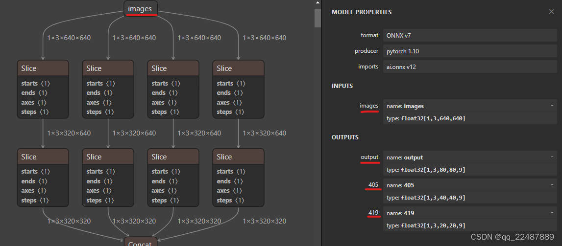
可以从ONNX 格式的模型看到数据的输入输出格式为：展示的是整个模型的所有输入输出节点，可以看到有一个输入（名称为images）和三个输出。实际部署的时候是导出的单输出模型，三个输出只是便于介绍。

输入格式：1x3x640x640，3是RGB三通道，总体是 Batch Channel H W。
输出有三层，分别在三个不同的位置，有不同的格式。

下面对其进行简单的解释。
在这里插入图片描述

标准的 yolov5 的输出有三个，分别是 1x255x80x80 1x255x40x40 1x255x20x20 其中这里的255是85*3，80×80、40×40 和 20×20 是特征图分辨率
这里的3是指3个锚框，而这里的85是指5+80=85，其中80是类别数量，每个类别数量对应一个label score,一共80个label score,而5是指box的四个坐标加一个box score.
三个输出层中浅层特征图分辨率是80乘80，中层是40乘40，深层是20乘20
一般来说浅层用于预测小物体，深层用于预测大物体。可以根据感受野的概念来理解。

上图的介绍：三输出模型的输出结果是 t_x t_y t_w t_h 和 t₀，即sigmoid之前的参数，单输出的模型直接输出的是 b_x b_y b_w b_h 和 score，即直接对应到原图中的坐标参数。
实际上单输出其实就是在导出模型的时候多做了 t_x t_y t_w t_h t₀ —–> b_x b_y b_w b_h score 的步骤，直接获取每个Anchor对于原图的信息，而不用自己进行复杂的处理，会非常有利于部署。
上图是YOLOV2 和 YOLOV3 的参数，YOLOV3 相对于YOLOV2的改进就是 objectness score 非0即1。

3.2 YOLOV4 和 V5 相对于 V2 V3 的改进

实际上在 YOLOV4 和 YOLOV5 中为了消除 Grid 敏感度，参数关系略有不同，如下图所示：这样可以取到 0 和 1。
YOLOV4：对 b_x b_y 的改进如下

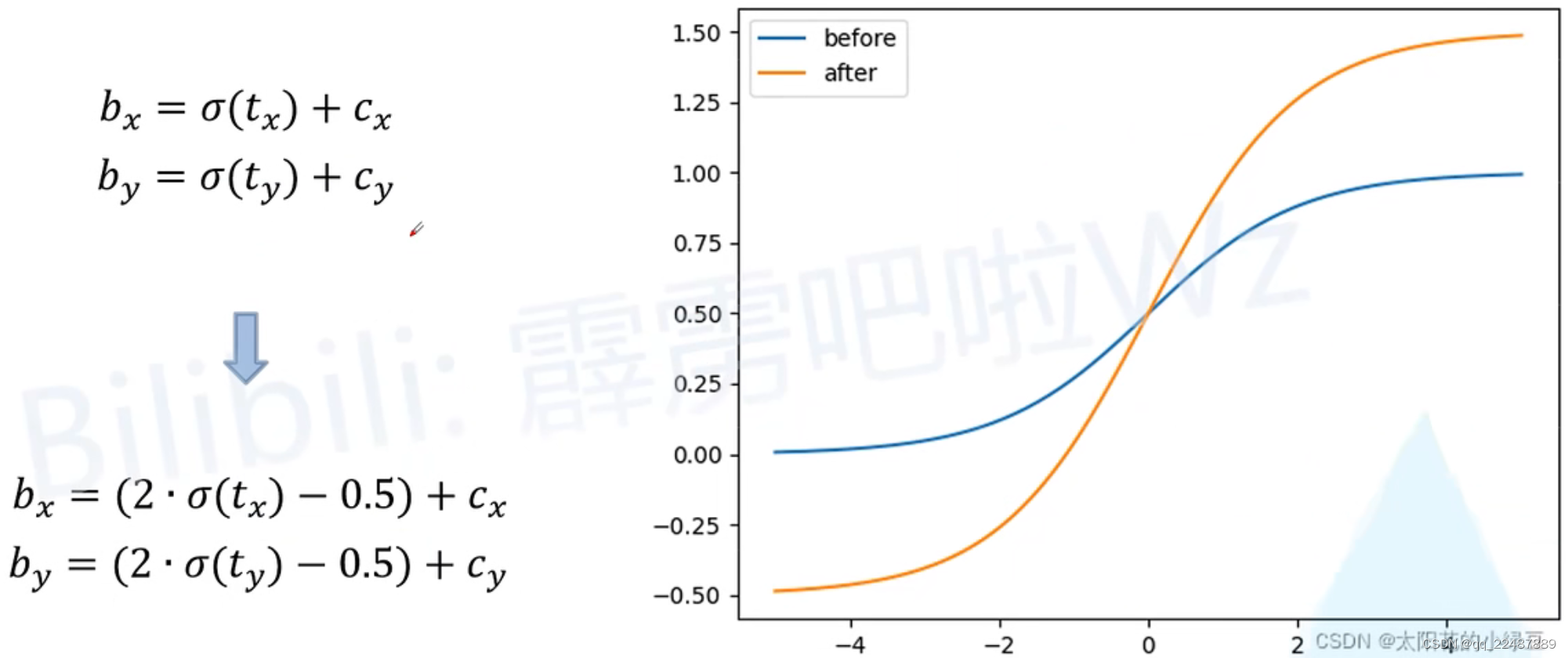
YOLOV5：在YOLOV4对对 b_x b_y 的改进基础上，对 b_w b_h进行了改进
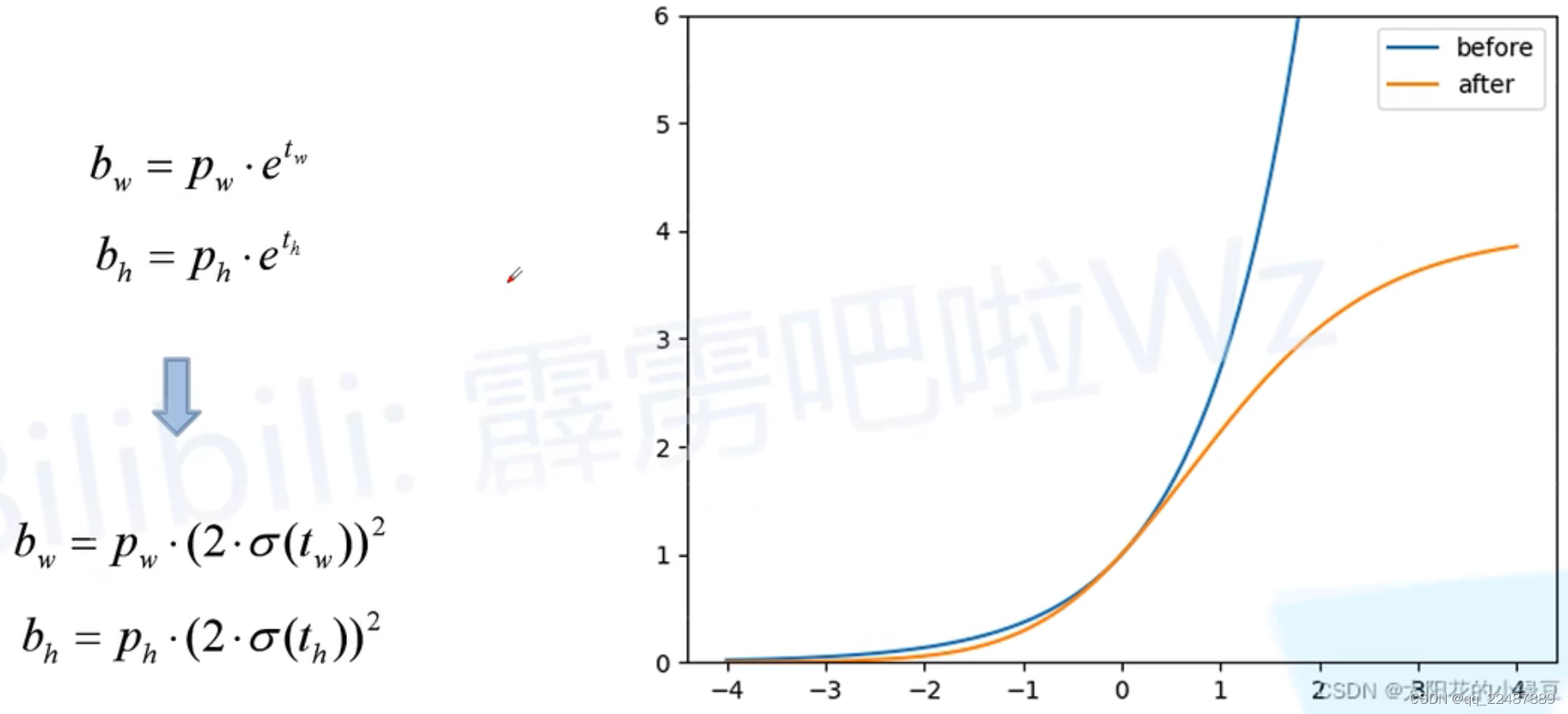
根据论文和代码，上面的虚线部分，在80×80；40×40 和 20×20 大小的输出中，锚框大小（p_w p_h）为：
[(10,13), (16,30), (33,23)] # 80×80的三个锚框
[(30,61), (62,45), (59,119)] # 40×40的三个锚框
[(116,90), (156,198), (373,326)] #20×20 的三个锚框
其损失函数是结合三层输出的损失值：

3.3 输入数据的处理

代码：

    def inference(self, img_path):
        """ 1.cv2读取图像并resize
        2.图像转BGR2RGB和HWC2CHW(因为yolov5的onnx模型输入为 RGB：1 × 3 × 640 × 640)
        3.图像归一化
        4.图像增加维度
        5.onnx_session 推理 """
        img = cv2.imread(img_path)
        or_img = cv2.resize(img, (640, 640))  # resize后的原图 (640, 640, 3)
        img = or_img[:, :, ::-1].transpose(2, 0, 1)  # BGR2RGB和HWC2CHW
        img = img.astype(dtype=np.float32)  # onnx模型的类型是type: float32[ , , , ]
        img /= 255.0
        img = np.expand_dims(img, axis=0)  # [3, 640, 640]扩展为[1, 3, 640, 640]
        # img尺寸(1, 3, 640, 640)
        input_feed = self.get_input_feed(img)  # dict:{ input_name: input_value }
        pred = self.onnx_session.run(None, input_feed)[0]  # <class 'numpy.ndarray'>(1, 25200, 9)

        return pred, or_img

把输入的图片转换成 1x3x640x640，再作为模型的输入：
opencv python 把图(cv2下)BGR转RGB，且HWC转CHW
如果想要使用可变的输入尺寸，参考下面yolov5的源码中的 padded resize 方法，检测效果其实更好：

detect.py:
dataset.py: class LoadImages:的函数

3.4 输出数据的处理

当输入图像是 640×640 时，输出数据是 (1, 25200, 4+1+class)：4+1+class 是检测框的坐标、大小和分数。导出为这种单输出，直接获得的就是每个预测框的 b_x b_y b_w b_h，而不是 Anchor 的 t_x t_y t_w t_h。

输出数据对应的位置是：0 – 8 对应的是 b_x b_y b_w b_h score + 每种类别的条件概率
进行置信度过滤、极大值抑制和坐标转换，即可得到结果了。
代码：

def filter_box(org_box, conf_thres, iou_thres):  # 过滤掉无用的框
    # -------------------------------------------------------
    #   删除为1的维度
    #	删除置信度小于conf_thres的BOX
    # -------------------------------------------------------
    org_box = np.squeeze(org_box)  # 删除数组形状中单维度条目(shape中为1的维度)
    # (25200, 9)
    # […,4]：代表了取最里边一层的所有第4号元素，…代表了对:,:,:,等所有的的省略。此处生成：25200个第四号元素组成的数组
    conf = org_box[..., 4] > conf_thres  # 0 1 2 3 4 4是置信度，只要置信度 > conf_thres 的
    box = org_box[conf == True]  # 根据objectness score生成(n, 9)，只留下符合要求的框
    print('box:符合要求的框')
    print(box.shape)

    # -------------------------------------------------------
    #   通过argmax获取置信度最大的类别
    # -------------------------------------------------------
    cls_cinf = box[..., 5:]  # 左闭右开（5 6 7 8），就只剩下了每个grid cell中各类别的概率
    cls = []
    for i in range(len(cls_cinf)):
        cls.append(int(np.argmax(cls_cinf[i])))  # 剩下的objecctness score比较大的grid cell，分别对应的预测类别列表
    all_cls = list(set(cls))  # 去重，找出图中都有哪些类别
    # set() 函数创建一个无序不重复元素集，可进行关系测试，删除重复数据，还可以计算交集、差集、并集等。
    # -------------------------------------------------------
    #   分别对每个类别进行过滤
    #   1.将第6列元素替换为类别下标
    #	2.xywh2xyxy 坐标转换
    #	3.经过非极大抑制后输出的BOX下标
    #	4.利用下标取出非极大抑制后的BOX
    # -------------------------------------------------------
    output = []
    for i in range(len(all_cls)):
        curr_cls = all_cls[i]
        curr_cls_box = []
        curr_out_box = []

        for j in range(len(cls)):
            if cls[j] == curr_cls:
                box[j][5] = curr_cls
                curr_cls_box.append(box[j][:6])  # 左闭右开，0 1 2 3 4 5

        curr_cls_box = np.array(curr_cls_box)  # 0 1 2 3 4 5 分别是 x y w h score class
        # curr_cls_box_old = np.copy(curr_cls_box)
        curr_cls_box = xywh2xyxy(curr_cls_box)  # 0 1 2 3 4 5 分别是 x1 y1 x2 y2 score class
        curr_out_box = nms(curr_cls_box, iou_thres)  # 获得nms后，剩下的类别在curr_cls_box中的下标

        for k in curr_out_box:
            output.append(curr_cls_box[k])
    output = np.array(output)
    return output

其中非极大值抑制 curr_out_box = nms(curr_cls_box, iou_thres) 和坐标转换 curr_cls_box = xywh2xyxy(curr_cls_box)：

# dets:  array [x,6] 6个值分别为x1,y1,x2,y2,score,class
# thresh: 阈值
def nms(dets, thresh):
    # dets:x1 y1 x2 y2 score class
    # x[:,n]就是取所有集合的第n个数据
    x1 = dets[:, 0]
    y1 = dets[:, 1]
    x2 = dets[:, 2]
    y2 = dets[:, 3]
    # -------------------------------------------------------
    #   计算框的面积
    #	置信度从大到小排序
    # -------------------------------------------------------
    areas = (y2 - y1 + 1) * (x2 - x1 + 1)
    scores = dets[:, 4]
    # print(scores)
    keep = []
    index = scores.argsort()[::-1]  # np.argsort()对某维度从小到大排序
    # [::-1] 从最后一个元素到第一个元素复制一遍。倒序从而从大到小排序

    while index.size > 0:
        i = index[0]
        keep.append(i)
        # -------------------------------------------------------
        #   计算相交面积
        #	1.相交
        #	2.不相交
        # -------------------------------------------------------
        x11 = np.maximum(x1[i], x1[index[1:]])
        y11 = np.maximum(y1[i], y1[index[1:]])
        x22 = np.minimum(x2[i], x2[index[1:]])
        y22 = np.minimum(y2[i], y2[index[1:]])

        w = np.maximum(0, x22 - x11 + 1)
        h = np.maximum(0, y22 - y11 + 1)

        overlaps = w * h
        # -------------------------------------------------------
        #   计算该框与其它框的IOU，去除掉重复的框，即IOU值大的框
        #	IOU小于thresh的框保留下来
        # -------------------------------------------------------
        ious = overlaps / (areas[i] + areas[index[1:]] - overlaps)
        idx = np.where(ious <= thresh)[0]
        index = index[idx + 1]
    return keep


def xywh2xyxy(x):
    # [x, y, w, h] to [x1, y1, x2, y2]
    y = np.copy(x)
    y[:, 0] = x[:, 0] - x[:, 2] / 2
    y[:, 1] = x[:, 1] - x[:, 3] / 2
    y[:, 2] = x[:, 0] + x[:, 2] / 2
    y[:, 3] = x[:, 1] + x[:, 3] / 2
    return y

识别结果如下：脱离Pytorch环境部署成功！如果对输入数据处理时，长宽比不变，效果会更好，如何处理参考 YOLOV5源码。
在这里插入图片描述

文章出处登录后可见！

已经登录？立即刷新

详细介绍 Yolov5 转 ONNX模型 + 使用ONNX Runtime 的 Python 部署（包含官方文档的介绍）