写在前面:好久没用到matplotlib,最近用到的时候发现有些点已经忘了还得查资料,所以趁此机会把matplotlib中常用到的画图方法总结一下!
matplotlib 官网
matplotlib是python中非常实用的一个模块,可以使用matplotlib绘制各种各样的图形,比如折线图、散点图、直方图、条形图、饼图、雷达图等。在python中安装和导入matplotlib包如下:
# 安装
pip install matplotlib
# 导入
import matplotlib.pyplot as plt
# 查看安装包的版本
matplotlib.__version__
一、matplotlib的图形构成
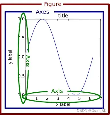
Figure:是指整个图形,也就是一张画布,包括了所有的元素,如标题,轴线等;
Axes:绘制 2D 图像的实际区域,也称为轴域区,或者绘图区;
Axis:是指图形的水平轴和垂直轴,包括轴的长度、轴的标签和轴的刻度等;
Artist:在画布上看到的所有元素都属于 Artist 对象,比如文本对象(title、xlabel、ylabel)、Line2D 对象(用于绘制2D图像)等。
Q:在画图时会经常遇到plt.plot 和ax.plot ,这两者的效果都是一样的,那么这两者有什么区别呢?
A:
figure 是上图中红色的外框,可以理解为一整张画布,而axes是蓝色的框,是画布中的一块子图,当需要画一张图形时,既可以用plt.plot()也可以用ax.plot()实现。
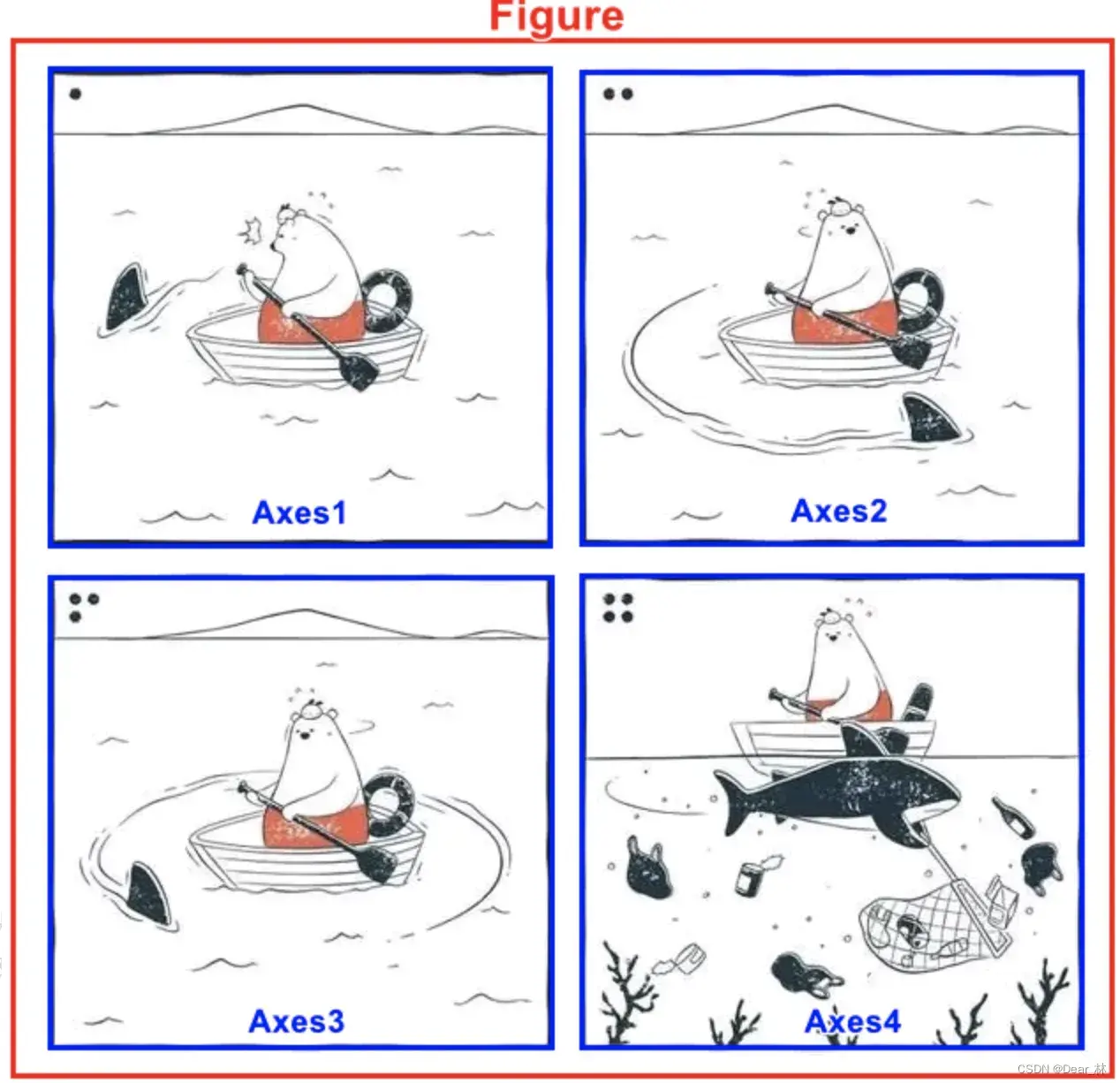
再比如上图,figure就是上图中的一整张画布,而Axes就是其中的子图,所以画图其实是在Axes上进行的。上图可以用一下代码来实现:
plt.figure()
plt.gcf.subplots(2,2)
.gcf() 就是获取当前的figure,即get current figure,另外 .gca() ,是获取当前的Axes,即get current axes.
另外 比如plt.plot()、plt.bar() 等,本质上还是在Axes上画图,可以理解为:现在figure上获取一个当前要操作的Axes,如果没有则自动创建一个并将其设置为当前的Axes,然后在这个Axes上执行当前的绘图操作,plt.xxx() 就相当于 plt.gca().xxx
二、绘制图形的各种要素
下面就从折线图说起,来了解绘制图形的各种要素
1、plt.figure()
在绘制图形时,首先用 plt.figure() 绘制一张画布 figure,可以将此figure命名为fig,此时的figure是空白的,后面可以在figure上绘制一个或者多个子图像。
用ax = fig.add_subplot() 向figure中添加Axes,并命名为ax,此后绘制子图就在ax中,就可以给子图ax设置各种属性。
例如:
# create data
A1 = np.arange(1, 6) # x ∈ [1,5]
A2 = np.arange(1, 11) # x ∈ [1,10]
B = A1 ** 2
C = A1 ** 3
D = A2 ** 2
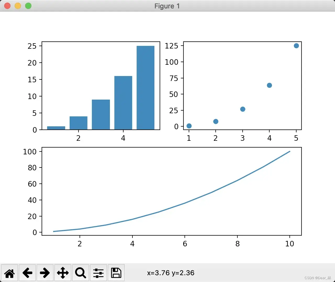
# create figure and axes
fig = plt.figure()
ax1 = fig.add_subplot(221)
ax2 = fig.add_subplot(222)
ax3 = fig.add_subplot(212)
# plot data
ax1.bar(A1, B)
ax2.scatter(A1, C)
ax3.plot(A2, D)
plt.show()
不过更好用的方法是 fig, axes = plt.subplots(),在创建画板的同时也将画布赋给了 axes,比上面的 add_subplot 要方便不少。
plt.figure() 调用方法:
plt.figure(num=None, figsize=None, dpi=None,
		   facecolor=None, edgecolor=None, frameon=True,
		   FigureClass=<class 'matplotlib.figure.Figure'>,
		   clear=False, **kwargs)
文档:链接
参数说明:
num:当给一个数字时,相当于figure的编号,相当于ID,当是字符串时,就作为figure的名称;
figsize:指定画布的大小,(宽度,高度),单位为英寸;
dpi:指定绘图对象的分辨率,即每英寸多少个像素,默认值为80;
facecolor:背景颜色;
edgecolor:边框颜色;
frameon:是否显示边框;
例如:
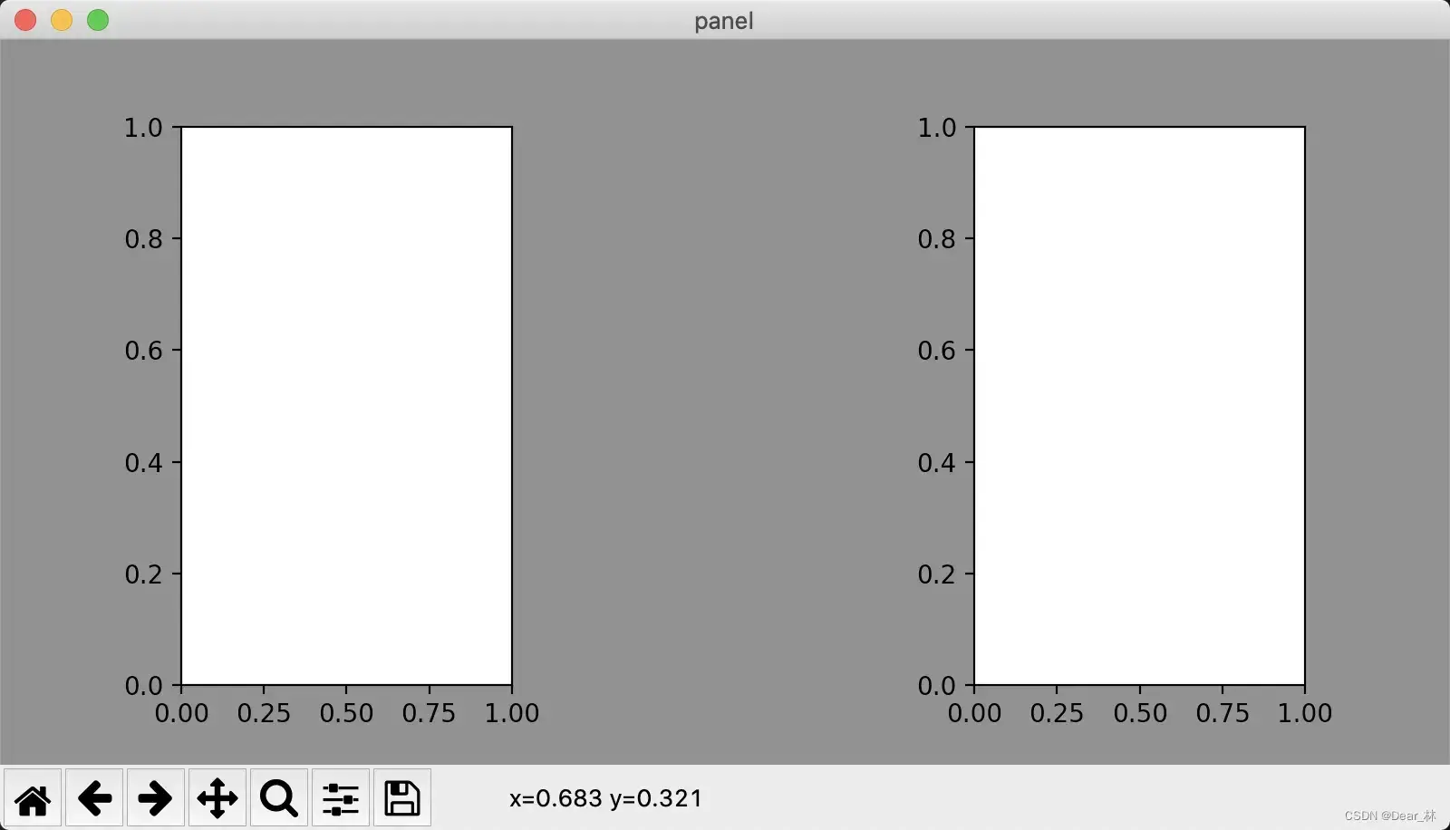
# 创建一个名为panel的figure,大小是3*2英寸,背景颜色时灰色
plt.figure(num='panel', figsize=(3,2),facecolor='gray')
plt.show()

2、plt.subplot()
当有一个空白画布时,可以用 subplot 划分多个子区域进行绘图。将画布整个区域分为 nrows 行,ncols 列,subplot 的 index 参数将指示当前绘制在第几个区域。区域编号的顺序从上之下,从左至右。
plt.subplot(nrows, ncols, index, **kwargs)
文档:链接
plt.figure(num='panel', figsize=(8,4),facecolor='gray')
# 划分三个小区域,绘制出第一个和第三个区域
plt.subplot(1,3,1)  # 划分1行3列,第1个子区域
plt.subplot(1,3,3)  # 划分1行3列,第3个子区域
plt.show()
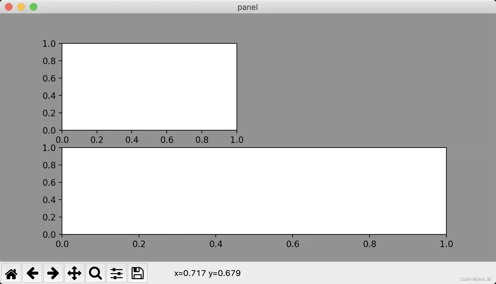
有时候需要绘制的子图大小是不一样的,这时就需要对figure进行多次划分,每一次划分后将子图安置在合适的位置即可。注意!前一次的划分是不影响后一次的划分,比如前一次将figure划分为22,不影响下一次将figure划分为21,只需要将子图安置在划分后的空白区域即可。
例如:
plt.figure(num='panel', figsize=(8,4),facecolor='gray')
plt.subplot(2,2,1)  # 划分2行2列,第1个子区域
plt.subplot(2,1,2)  # 划分2行1列,第2个子区域
plt.show()
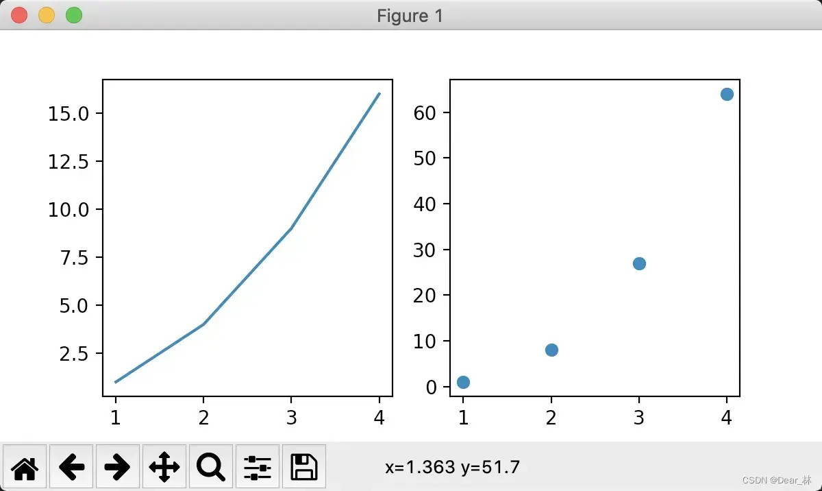
4、plt.subplots()
最常用的就是 subplots,便于绘图时精调细节信息。如果用 subplots 创建了多个子图,那么 axes 就是一个 list,用索引列表元素的方法就能获取到每一个 axes。
# create data
A = np.arange(1,5)
B = A**2
C = A**3

# create figure and axes
fig, axes = plt.subplots(1, 2, figsize=(6,3))

# plot data
axes[0].plot(A,B)
axes[1].scatter(A,C)
plt.show()
由于axes是list,可以通过索引,因此也可以在循环中使用。
4、使用matplotlib的两种方法
通过上面的了解,可看出对matplotlib的使用有两种基本的方法:
1⃣️创建figure和axes,并在其上面调用方法(面向对象方法 object-oriented (OO) style);
2⃣️通过pyplot创建和管理图形和轴,并使用pyplot函数进行绘图;
下面来通过一个栗子来说明一下:
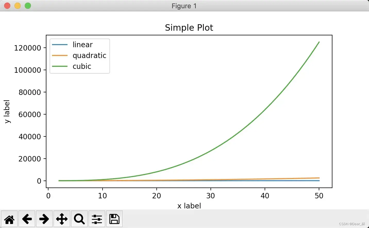
# 使用OO模式绘图
x = np.linspace(2, 50, 100)
fig, ax = plt.subplots(figsize=(6, 5))
ax.plot(x, x, label='linear')
ax.plot(x, x**2, label='quadratic')
ax.plot(x, x**3, label='cubic')
# 设置x,y轴的标签
ax.set_xlabel('x label')
ax.set_ylabel('y label')
# 设置ax的标签
ax.set_title("Simple Plot")
ax.legend()
# 使用pyplot函数绘图
x = np.linspace(2, 50, 100)
plt.figure(figsize=(6, 5))
plt.plot(x, x, label='linear')
plt.plot(x, x**2, label='quadratic')
plt.plot(x, x**3, label='cubic')

# 设置x,y轴的标签
plt.xlabel('x label')
plt.ylabel('y label')

# 设置标签
plt.title('Simple Plot')
# 设置标签的位置
plt.legend()
plt.show()
输出结果如下:
5、润色绘制的图表
绘制的图表为了更加的通俗易懂以及美观,需要在绘制的图表上添加一些配置;以折线图为例,可是设置图片的大小,x、y轴的描述信息,调整x、y轴的刻度,线条的样式(颜色、透明度),标记出特殊的点,将绘制的图片保存到本地,给图片添加一个水印等。下面依次来看一下这些方法要如何实现。
设置图片的大小和保存图片
# 绘制数据
x = np.arange(2, 26, 2)
y = [15, 13, 14.5, 17, 20, 20.5, 26, 26, 24, 22, 18, 15]

### 方法一:使用pyplot
# 设置图片的大小和像素
plt.figure(figsize=(6, 5), dpi=90)
plt.plot(x, y)
# 保存图片
plt.savefig('./sig_size.png')   # 这里需要注意的是保存图片要在plt.show()之前
plt.show()

### 方法二:OO style
# 设置图片的大小
fig, ax = plt.subplots(figsize=(5, 6))
ax.plot(x, y)
# 保存图片
fig.savefig('./sig_si.png')
# 显示图片
plt.show()
x、y轴的标签及刻度
通过一个栗子来了解一下如何实现:
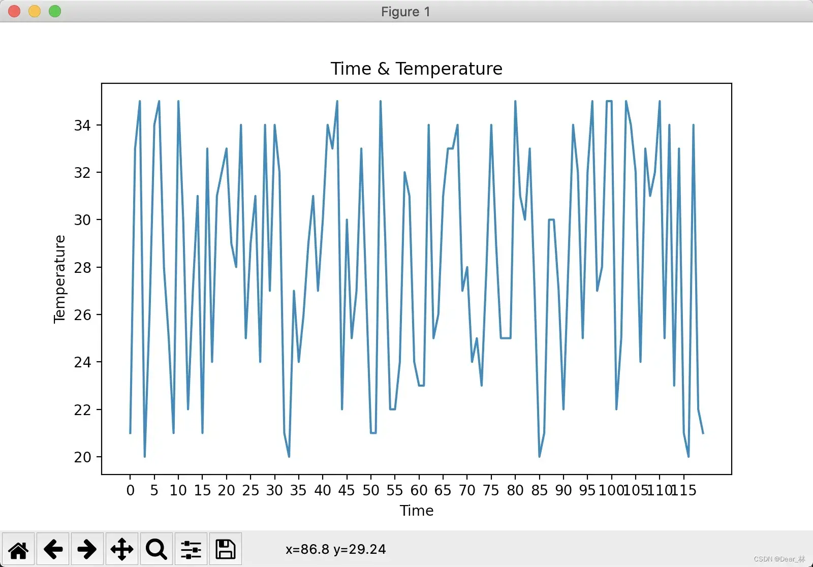
例:列表a表示10点到12点的每一分钟的气温,如何用折线图绘制气温的变化,a = [random.randint(20, 35) for i in range(120)]
# 方法一:
# 设置随机种子,让不同时间得到的随机结果都是一样的
random.seed(10)
x = range(120)
y = [random.randint(20, 35) for i in range(120)]
plt.figure(figsize=(12, 8))
plt.plot(x, y)
# 设置坐标轴的标签
plt.xlabel('Time')
plt.ylabel('Temperature')

# 设置图片标题
plt.title('Time & Temperature')
# 为了简洁,可以等间隔的设置x轴的刻度
plt.xticks(x[::5])
plt.show()

# 方法二:
fig, ax = plt.subplots(figsize=(8, 5))
ax.plot(x, y)
# 设置坐标轴的标签
ax.set_xlabel('Time')
ax.set_ylabel('Temperature')

# 设置标题
ax.set_title('Time & Temperature')

# 设置刻度
ax.set_xticks(x[::5])
plt.show()
绘图结果:
从上面的展示结果可看出,x轴的刻度的并没有表示出时间的变化,下面就对x轴的刻度做一个修改并用中文显示;
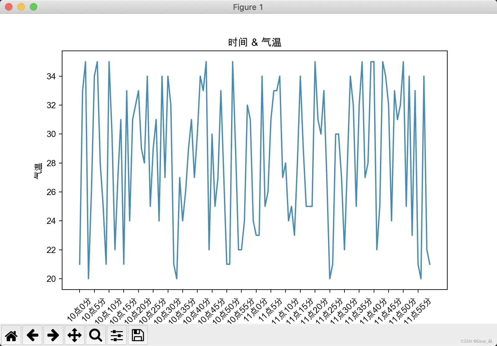
显示中文
在图标上显示中文,最简单的方法是添加下面一行代码
plt.rcParams['font.sans-serif'] = ['Arial Unicode MS']
random.seed(10)
x = range(120)
y = [random.randint(20, 35) for i in range(120)]
plt.figure(figsize=(8, 5))
plt.plot(x, y)
# 设置坐标轴的标签
plt.xlabel('时间')
plt.ylabel('气温')

# 设置图片标题
plt.title('时间 & 气温')
# 为了简洁,可以等间隔的设置x轴的刻度
_xticks = ['10点{}分'.format(i) for i in range(60)]
_xticks += ['11点{}分'.format(i) for i in range(60)]
# 这里需要注意的是列表x的数据和_xticks的数据要对应上,会在x轴上一一对应显示出来,两组数据的长度要一致
plt.xticks(x[::5], _xticks[::5], rotation=45) # 为了将x轴的刻度显示清晰明确,可以将刻度标签旋转一定的角度
plt.show()
输出结果:
设置线条的风格
在上面绘制出的图标中线条的颜色和样式都是默认的,也可以自定义线条的风格。
线条的属性
| 线条风格linestyle或ls | 描述 |
|---|---|
| – | 实线 |
| – | 破折线 |
| -. | 点划线 |
| : | 虚线 |
| ’ ’ | 留空或空格,无线条 |
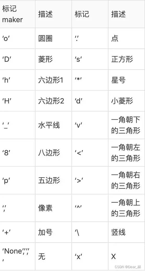
线条标记
颜色标记
可以通过调用matplotlib.pyplot.colors()得到matplotlib支持的所有颜色。
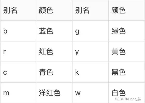
如果这两种颜色不够用,还可以通过两种其他方式来定义颜色值:
1⃣️使用HTML十六进制字符串 color=‘eeefff’ 使用合法的HTML颜色名字(’red’,’chartreuse’等)。
2⃣️也可以传入一个归一化到[0,1]的RGB元祖。 color=(0.3,0.3,0.4)
一句话总结就是:
color©颜色
marker标记,markersize为标记大小
linestyle(ls)线样式,linewidth线宽
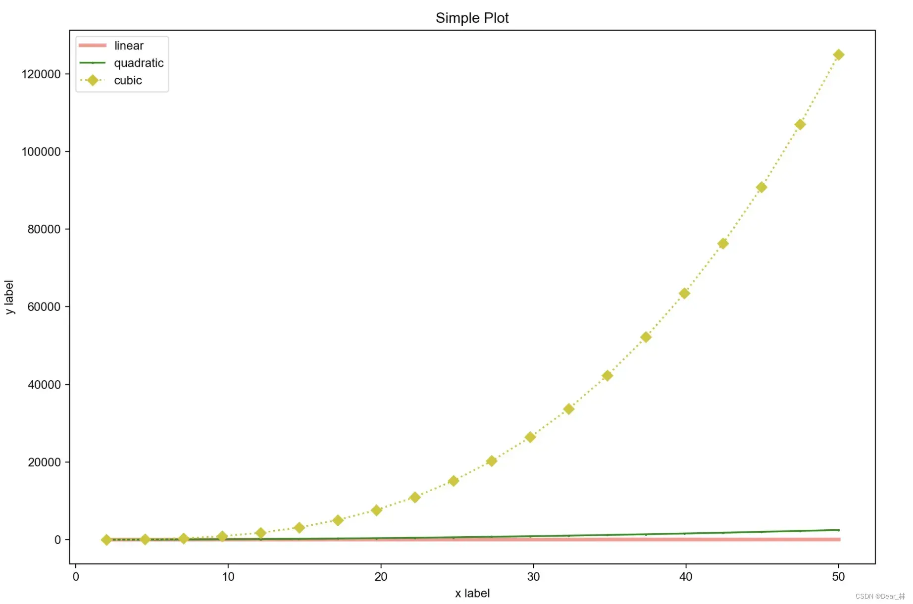
例如:
x = np.linspace(2, 50, 20)
plt.figure(figsize=(12, 8))
# 设置线条的标签,颜色,风格,粗细,透明度
plt.plot(x, x, label='linear', color='r', linestyle='-', linewidth=3, alpha=0.5)
# 线条颜色,风格,标记的不同设置方法
plt.plot(x, x**2, label='quadratic', c='green', ls='-', marker='o', markersize=1)
# 三合一
plt.plot(x, x**3, 'y:D', label='cubic')

# 设置x,y轴的标签
plt.xlabel('x label')
plt.ylabel('y label')

# 设置标签
plt.title('Simple Plot')
# 设置标签的位置
plt.legend()
plt.show()
输出结果:
在上面例子中出现的plt.legend()是设置线条标签的位置,plt.legend( )中有handles、labels和loc三个参数,其中:
handles:传入所画线条的实例对象;
labels:labels是图例的名称(能够覆盖在plt.plot( )中label参数值)
loc:图例在整个坐标轴平面中的位置(一般选取’best’这个参数值)
关于loc参数的选择有几种方法:
方法一:默认best
图例会自动放置在图表中数据较少的位置
方法二:loc = ‘XXX’
可选择的参数也有一下几种
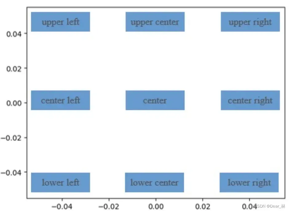
方法三:loc=(x,y)
(x, y)表示图例左下角的位置,这是最灵活的一种放置图例的方法
关于如何控制loc的位置,可以参数这篇文章:链接
其它设置
设置网格线:plt.grid()
给图片添加水印:
1⃣️添加图片水印:plt.figimage() fig.figimage()
2⃣️添加文本水印:plt.figtext() fig.text()
添加注释:plt.annotate()
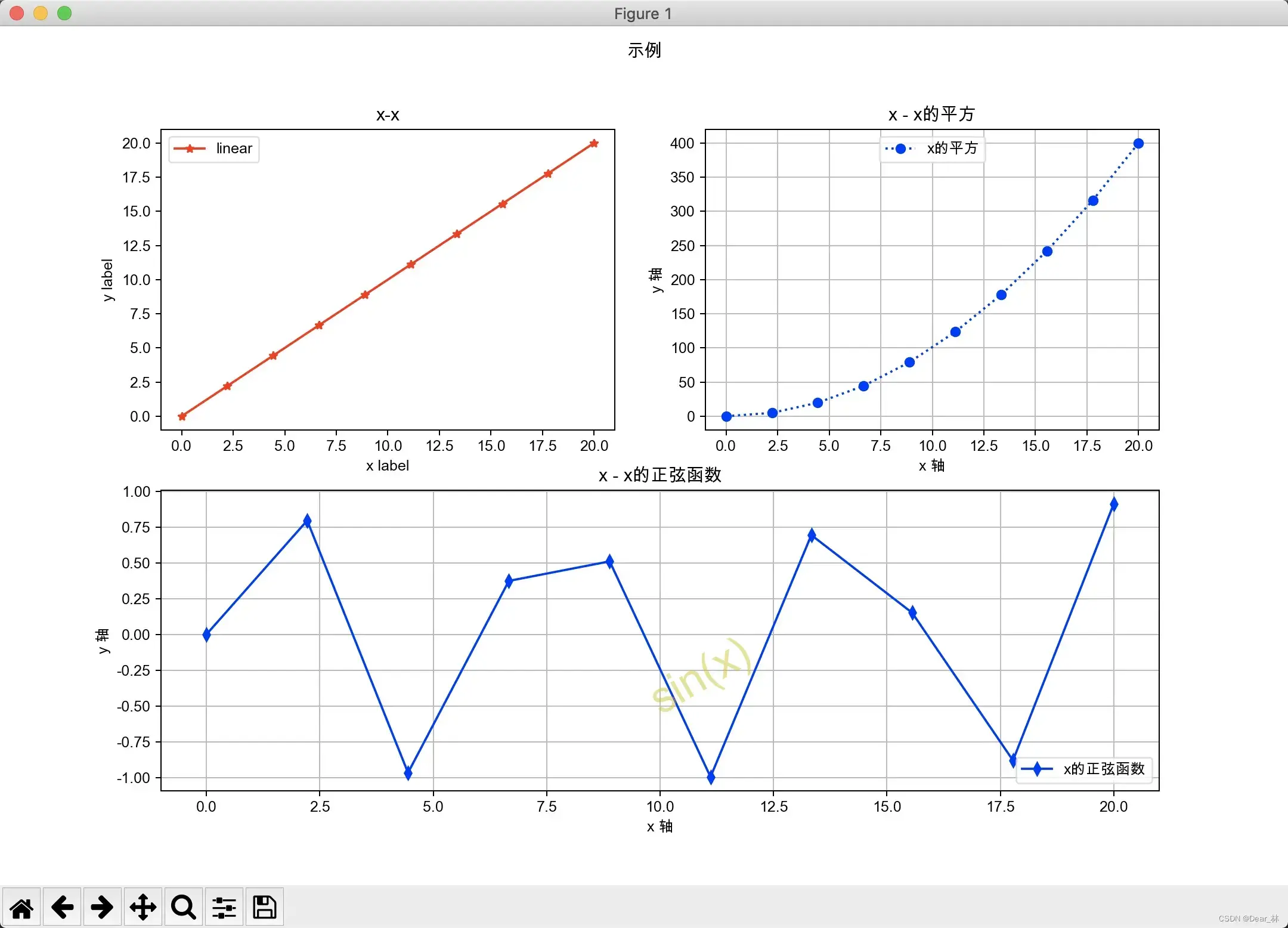
下面就以一张figure上绘制多张子图为例,总结一下上面列举到的所有方法
# 方法一:
x = np.linspace(0, 20, 10)
plt.figure(figsize=(12, 8), dpi=90)
plt.subplot(221)
plt.plot(x, x, label='linear', color='r', linestyle='-', marker='*')
plt.xlabel('x label')
plt.ylabel('y label')
plt.title('x-x')
plt.legend()

plt.subplot(222)
plt.plot(x, x**2, label='x的平方', color='#0000FF', linestyle=':', marker='o')
plt.xlabel('x 轴')
plt.ylabel('y 轴')
plt.title('x - x的平方')
plt.grid()
plt.legend(loc='upper center')

plt.subplot(212)
plt.plot(x, np.sin(x), 'b-d', label='x的正弦函数')
plt.xlabel('x 轴')
plt.ylabel('y 轴')
plt.title('x - x的正弦函数')
plt.grid()
plt.legend(loc='lower right')
plt.figtext(0.5, 0.2, 'sin(x)', alpha=0.5, rotation=30, color='y', size=30)

plt.suptitle('示例')
plt.show()
x = np.linspace(0, 20, 10)
# plt.figure(figsize=(12, 8), dpi=90)
fig = plt.figure(figsize=(12, 8), dpi=90)
ax1 = fig.add_subplot(221)
ax1.plot(x, x, label='linear', color='r', linestyle='-', marker='*')
ax1.set_xlabel('x label')
ax1.set_ylabel('y label')
ax1.set_title('x-x')
ax1.legend()

ax2 = fig.add_subplot(222)
ax2.plot(x, x**2, label='x的平方', color='#0000FF', linestyle=':', marker='o')
ax2.set_xlabel('x 轴')
ax2.set_ylabel('y 轴')
ax2.set_title('x - x的平方')
ax2.grid()
ax2.legend(loc='upper center')

ax3 = fig.add_subplot(212)
ax3.plot(x, np.sin(x), 'b-d', label='x的正弦函数')
ax3.set_xlabel('x 轴')
ax3.set_ylabel('y 轴')
ax3.set_title('x - x的正弦函数')
ax3.grid()
ax3.legend(loc='lower right')

fig.text(0.5, 0.2, 'sin(x)', alpha=0.5, rotation=30, color='y', size=30)
fig.suptitle('示例')
plt.show()
输出结果:
三、散点图
直接通过一个例子来说明一下:
假设获取到了北京2016年3,10月份每天白天的最高气温(分别位于列表a,b),那么此时如何寻找出气温和随时间(天)变化的某种规律?
a = [11,17,16,11,12,11,12,6,6,7,8,9,12,15,14,17,18,21,16,17,20,14,15,15,15,19,21,22,22,22,23]
b = [26,26,28,19,21,17,16,19,18,20,20,19,22,23,17,20,21,20,22,15,11,15,5,13,17,10,11,13,12,13,6]
分析:用散点图横轴表示日期,纵轴表示温度
y_3 = [11,17,16,11,12,11,12,6,6,7,8,9,12,15,14,17,18,21,16,17,20,14,15,15,15,19,21,22,22,22,23]
y_10 = [26,26,28,19,21,17,16,19,18,20,20,19,22,23,17,20,21,20,22,15,11,15,5,13,17,10,11,13,12,13,6]

x_3 = range(1, 32)
x_10 = range(51, 82)

# 设置图形大小
plt.figure(figsize=(12, 5), dpi=90)
# 绘图
plt.scatter(x_3, y_3, label='3月份', color='r', marker='D')
plt.scatter(x_10, y_10, label='10月份', color='y', marker='*')
# 调整x轴的刻度
_x = list(x_3) + list(x_10)
_xtick_label = ['3月{}日'.format(i) for i in x_3]
_xtick_label += ['10月{}日'.format(i-50) for i in x_10]
plt.xticks(_x[::3], _xtick_label[::3], rotation=45)

# 添加图例
plt.legend(loc='upper right')

# 添加描述信息
plt.xlabel('时间')
plt.ylabel('温度')
plt.title('时间 & 温度')

# 展示
plt.show()
输出结果:
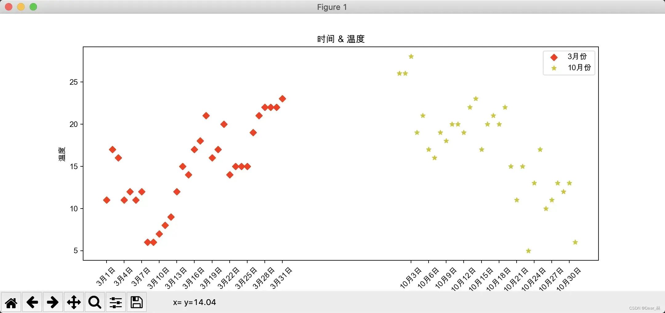
离散图的应用场景:
- 不同条件(维度)之前的内在关联关系;
- 观察数据的离散聚合程度;
四、条形图
还是通过一个例子来看一下:
从某网站获取到了2017年内地电影票房前20的电影(列表a)和电影票房数据(列表b),那么如何更加直观的展示该数据?(数据地址:链接)
a = [“战狼2”,“速度与激情8”,“功夫瑜伽”,“西游伏妖篇”,“变形金刚5:最后的骑士”,“摔跤吧!爸爸”,“加勒比海盗5:死无对证”,“金刚:骷髅岛”,“极限特工:终极回归”,“生化危机6:终章”,“乘风破浪”,“神偷奶爸3”,“智取威虎山”,“大闹天竺”,“金刚狼3:殊死一战”,“蜘蛛侠:英雄归来”,“悟空传”,“银河护卫队2”,“情圣”,“新木乃伊”,]
b=[56.01,26.94,17.53,16.49,15.45,12.96,11.8,11.61,11.28,11.12,10.49,10.3,8.75,7.55,7.32,6.99,6.88,6.86,6.58,6.23] 单位:亿
a = ["战狼2","速度与激情8","功夫瑜伽","西游伏妖篇","变形金刚5:最后的骑士","摔跤吧!爸爸","加勒比海盗5:死无对证","金刚:骷髅岛",\
         "极限特工:终极回归","生化危机6:终章","乘风破浪","神偷奶爸3","智取威虎山","大闹天竺","金刚狼3:殊死一战","蜘蛛侠:英雄归来",\
         "悟空传","银河护卫队2","情圣","新木乃伊",]
b = [56.01,26.94,17.53,16.49,15.45,12.96,11.8,11.61,11.28,11.12,10.49,10.3,8.75,7.55,7.32,6.99,6.88,6.86,6.58,6.23]

plt.figure(figsize=(12, 8), dpi=90)
plt.bar(range(len(a)), b, width=0.3, color='orange')
plt.xticks(range(len(a)), a, rotation=90)
plt.xlabel('电影名称')
plt.ylabel('票房')
plt.grid()
# plt.savefig('./movie.png')
plt.show()
输出结果:
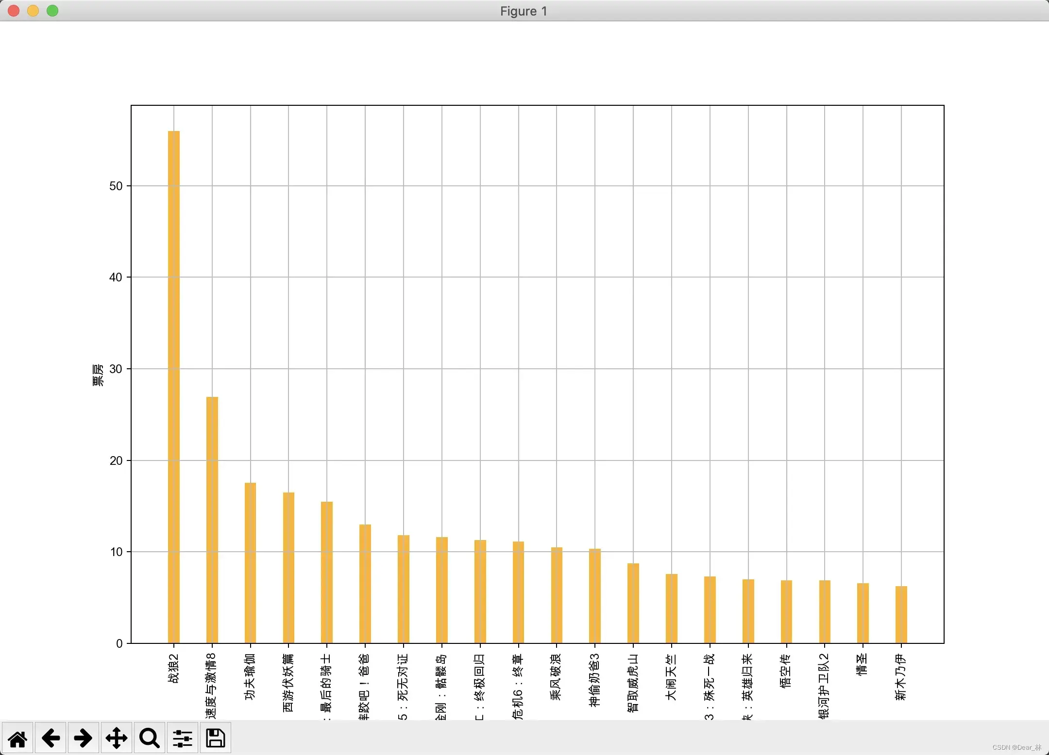
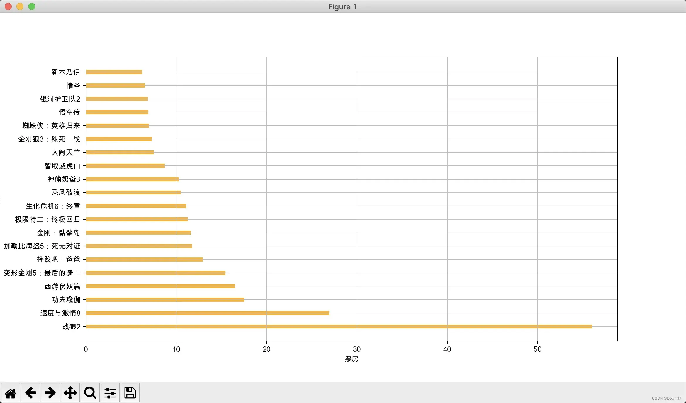
可看出横轴的电影名称显示不全,在这种情况下可以将条形图横置。
plt.figure(figsize=(13, 7), dpi=90)
plt.barh(range(len(a)), b, height=0.3, color='orange')
plt.yticks(range(len(a)), a)
plt.xlabel('票房')
plt.ylabel('电影名称')
plt.grid()
# plt.savefig('./movie.png')
plt.show()
输出结果:
这里需要注意的是 plt.bar() 和plt.barh() 各参数的设置上有些不同。
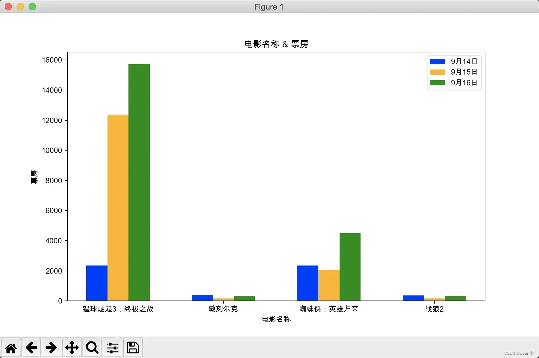
下面再来看一个例子来绘制多次条形图
列表a中电影分别在2017-09-14(b_14), 2017-09-15(b_15), 2017-09-16(b_16)三天的票房,为了展示列表中电影本身的票房以及同其他电影的数据对比情况,应该如何更加直观的呈现该数据?
a = [“猩球崛起3:终极之战”,“敦刻尔克”,“蜘蛛侠:英雄归来”,“战狼2”]
b_16 = [15746,312,4497,319]
b_15 = [12357,156,2045,168]
b_14 = [2358,399,2358,362]
a = ["猩球崛起3:终极之战", "敦刻尔克", "蜘蛛侠:英雄归来", "战狼2"]
b_16 = [15746, 312, 4497, 319]
b_15 = [12357, 156, 2045, 168]
b_14 = [2358, 399, 2358, 362]

plt.figure(figsize=(10, 6), dpi=90)
bar_width = 0.2
plt.bar(range(len(a)), b_14, width=bar_width, color='blue', label='9月14日')
# 这里需要注意的是x轴的值要跟上一个条形图紧挨着
plt.bar([i+bar_width for i in range(len(a))], b_15, width=bar_width, color='orange', label='9月15日')
plt.bar([i+2*bar_width for i in range(len(a))], b_16, width=bar_width, color='green', label='9月16日')
plt.xticks([i+bar_width for i in range(len(a))], a)
plt.xlabel('电影名称')
plt.ylabel('票房')
plt.title('电影名称 & 票房')
plt.legend()
plt.show()
输出结果:
条形图的适用场景:
- 数量统计;
- 频率统计;
五、直方图
还是通过一个例子来了解一下
栗子:
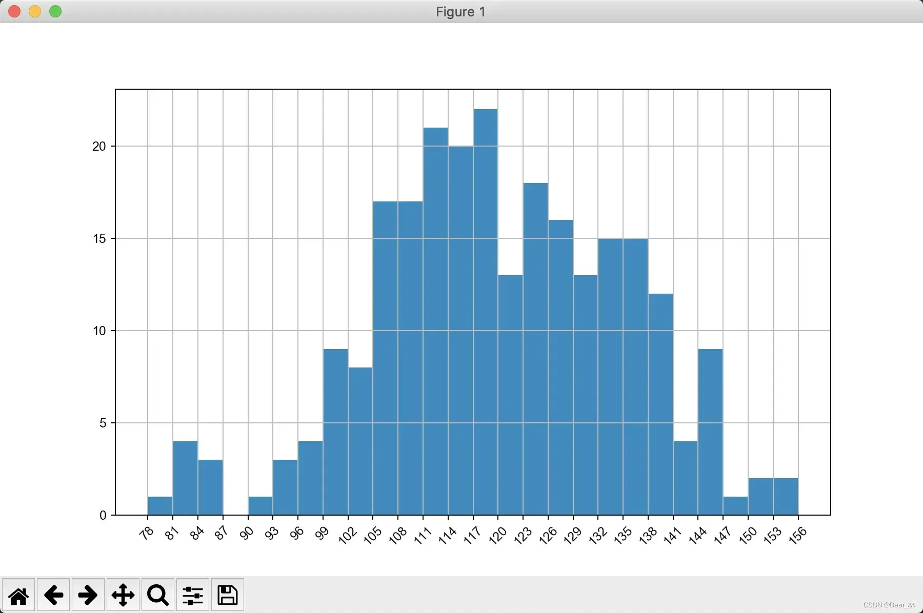
假设获取了250部电影的时长(列表a中),希望统计出这些电影时长的分布状态(比如时长为100分钟到120分钟电影的数量,出现的频率)等信息,应该如何呈现这些数据?
a=[131, 98, 125, 131, 124, 139, 131, 117, 128, 108, 135, 138, 131, 102, 107, 114, 119, 128, 121, 142, 127, 130, 124, 101, 110, 116, 117, 110, 128, 128, 115, 99, 136, 126, 134, 95, 138, 117, 111,78, 132, 124, 113, 150, 110, 117, 86, 95, 144, 105, 126, 130,126, 130, 126, 116, 123, 106, 112, 138, 123, 86, 101, 99, 136,123, 117, 119, 105, 137, 123, 128, 125, 104, 109, 134, 125, 127,105, 120, 107, 129, 116, 108, 132, 103, 136, 118, 102, 120, 114,105, 115, 132, 145, 119, 121, 112, 139, 125, 138, 109, 132, 134,156, 106, 117, 127, 144, 139, 139, 119, 140, 83, 110, 102,123,107, 143, 115, 136, 118, 139, 123, 112, 118, 125, 109, 119, 133,112, 114, 122, 109, 106, 123, 116, 131, 127, 115, 118, 112, 135,115, 146, 137, 116, 103, 144, 83, 123, 111, 110, 111, 100, 154,136, 100, 118, 119, 133, 134, 106, 129, 126, 110, 111, 109, 141,120, 117, 106, 149, 122, 122, 110, 118, 127, 121, 114, 125, 126,114, 140, 103, 130, 141, 117, 106, 114, 121, 114, 133, 137, 92,121, 112, 146, 97, 137, 105, 98, 117, 112, 81, 97, 139, 113,134, 106, 144, 110, 137, 137, 111, 104, 117, 100, 111, 101, 110,105, 129, 137, 112, 120, 113, 133, 112, 83, 94, 146, 133, 101,131, 116, 111, 84, 137, 115, 122, 106, 144, 109, 123, 116, 111,111, 133, 150]
分析:
绘制直方图之前,应该先将数据进行分组统计。那要如何进行分组呢?即要确定组数和组距,组数要选择适当,太多误差较大,太少规律不明显。
组数:将数据分组,当数据在100以内时,按数据多少常分为5-12组;
组距:每个小组两个端点之间的距离;
组数 = 极差/组距 极差=最大值-最小值
a = [131, 98, 125, 131, 124, 139, 131, 117, 128, 108, 135, 138, 131, 102, 107, 114, 119, 128, 121, 142, 127, 130,
     124, 101, 110, 116, 117, 110, 128, 128, 115, 99, 136, 126, 134, 95, 138, 117, 111, 78, 132, 124, 113, 150, 110,
     117, 86, 95, 144, 105, 126, 130, 126, 130, 126, 116, 123, 106, 112, 138, 123, 86, 101, 99, 136, 123, 117, 119,
     105, 137, 123, 128, 125, 104, 109, 134, 125, 127, 105, 120, 107, 129, 116, 108, 132, 103, 136, 118, 102, 120,
     114, 105, 115, 132, 145, 119, 121, 112, 139, 125, 138, 109, 132, 134, 156, 106, 117, 127, 144, 139, 139, 119,
     140, 83, 110, 102, 123, 107, 143, 115, 136, 118, 139, 123, 112, 118, 125, 109, 119, 133, 112, 114, 122, 109,
     106, 123, 116, 131, 127, 115, 118, 112, 135, 115, 146, 137, 116, 103, 144, 83, 123, 111, 110, 111, 100, 154,
     136, 100, 118, 119, 133, 134, 106, 129, 126, 110, 111, 109, 141, 120, 117, 106, 149, 122, 122, 110, 118, 127,
     121, 114, 125, 126, 114, 140, 103, 130, 141, 117, 106, 114, 121, 114, 133, 137, 92, 121, 112, 146, 97, 137,
     105, 98, 117, 112, 81, 97, 139, 113, 134, 106, 144, 110, 137, 137, 111, 104, 117, 100, 111, 101, 110, 105, 129,
     137, 112, 120, 113, 133, 112, 83, 94, 146, 133, 101, 131, 116, 111, 84, 137, 115, 122, 106, 144, 109, 123, 116,
     111, 111, 133, 150]
plt.figure(figsize=(10, 6), dpi=90)
# 确定组数和组距
bin_width = 3
bin_num = (max(a)-min(a))//bin_width
# 传入需要统计的数据以及组数
plt.hist(a, bin_num)
# 设置不等间隔的组距
# plt.hist(a, [min(a)+i*bin_width for i in range(bin_num)])

# 注意刻度的选择,设置不等间隔的组距时刻度也要对应上
plt.xticks(list(range(min(a), max(a)+bin_width))[::bin_width], rotation=45)
plt.grid()
plt.show()
输出结果:
六、饼图
直接上栗子:
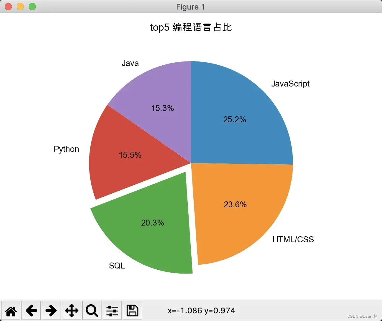
languages = ['JavaScript', 'HTML/CSS', 'SQL', 'Python', 'Java']
popularity = [59219, 55466, 47544, 36443, 35917]

plt.pie(popularity, labels=languages, autopct='%1.1f%%',
       counterclock=False, startangle=90,explode=[0,0,0.1,0,0])
# label:各区域的标签;autopct:各区域所占的百分比;
# 设置counterclock为False,是将区域从大到小顺时针排列,startangle=90将最大的扇形区域放置在12点钟的方向
# 为了突出某一个区域,设置explode参数

plt.title('top5 编程语言占比')
plt.tight_layout()
plt.show()
输出结果:
饼图适用场景:
想要突出表示某个部分在整体中所占比例,尤其该部分所占比例达到总体的25%或50%时。
分类数量最好小于5个。
各不同分类间的占比差异明显。
需要确定的图表绘制空间大小(不会随着分类增多有增大画布空间)。
七、其他绘图工具
以上是matplotlib的几种常用的图标,还可以绘制各钟图标:详情可见官网。
还有基于matplotlib的seaborn绘图工具包;
pyecharts 百度开源的数据可视化包:链接
文章出处登录后可见!