**
Faster-RCNN是多阶段目标检测算法RCNN系列中的集大成者,下面来看看分别看看这个系列的算法细节。
代码github地址:https://github.com/chenyuntc/simple-faster-rcnn-pytorch(非本人所写,只是个人觉得代码比较简洁,非常适合新手阅读)
**
**注:只简单讲解RCNN,Fast-RCNN算法。后面会重点讲解Fater-RCNN算法。
一、RCNN
RCNN是2013年出现的目标检测算法,首先将深度学习引 入目标检测领域 , m A P 由 D P M 的 3 5 . 1 提 升 至 53.7。
示意图如下:
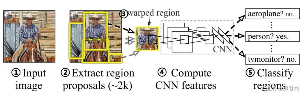
具体步骤如下:
①首先准备一张输入图片;
②候选区域生成:使用Selective Search算法,在输入图像上生成~2K个候选区域;
什么是Selective Search算法?
Selective Search算法:利用图像分割产生初始分割区域 -> 利用相似度进行区域合并
如何计算两个区域的相似度?
计算颜色、纹理、大小和形状交叠的差异,利用不同的权重相加
③ 候选区域处理:在输入图像上裁剪出每个候选区域,并缩放到227*227大小;
④ 特征提取:每个候选区域输入CNN网络提取一定维度(如4096维)的特征;
⑤ 类别判断:把提取的特征送入每一类的SVM 分类器,判别是否属于该类;
⑥ 位置精修:使用回归器精细修正候选框位置。
存在的问题:耗时。尽管RCNN算法已经比传统算法快了不少,但是由于其在候选区域生成上非常耗时以及要把2k+候选区域分别送入CNN网络进行特征提取,存在大量重复计算。特征提取、图像分类、边框回归是三个独立的步骤,要分别训练,测试效率也较低。
变形。将候选区域缩放到固定大小的时候容易产生形变,纵横比特征的丢失。
二、Fast -RCNN
Fast -RCNN是在RCNN基础上进行改进的一种算法。如图:
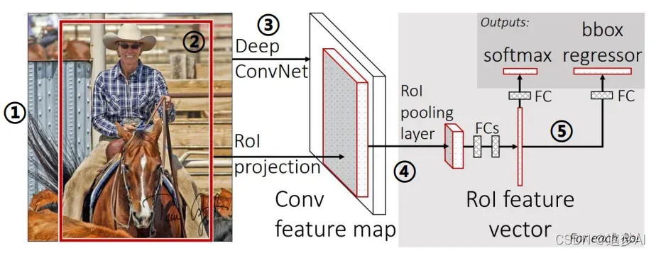
相比于RCNN算法,Fast R-CNN算法在前期改动并不大,依旧是使用SS算法去生成候选区域,不过在后续采用了RoIPooling去生成每个区域的特征。并直接对这些特征进行分类和回归。
具体检测步骤如下:
① 输入图像:输入一张待检测的图像;
② 候选区域生成:使用Selective Search算法,在输入图像上生成~2K个候选区域;
③ 特征提取:将整张图像传入CNN提取特征;
④ 候选区域特征:利用RoIPooling分别生成每个候选区域的特征;
⑤ 候选区域分类和回归:利用扣取的特征,对每个候选区域进行分类和回归。
*** 注:步骤④⑤仍会存在一些重复计算,但是相对R-CNN少了很多**
在了解了Fast RCNN的具体检测步骤之后,相信大家都会有一个问题,就是什么是RoIPooling?它在算法中起到了什么作用?下面来具体聊一聊。
还记得在RCNN中,是将图像中的2k+个候选区域,分别送入CNN去提取特征,并且要把这些候选区域都缩放至固定大小,这在网络中是非常耗时的,针对这一现象,在Fast RCNN中做了改进。
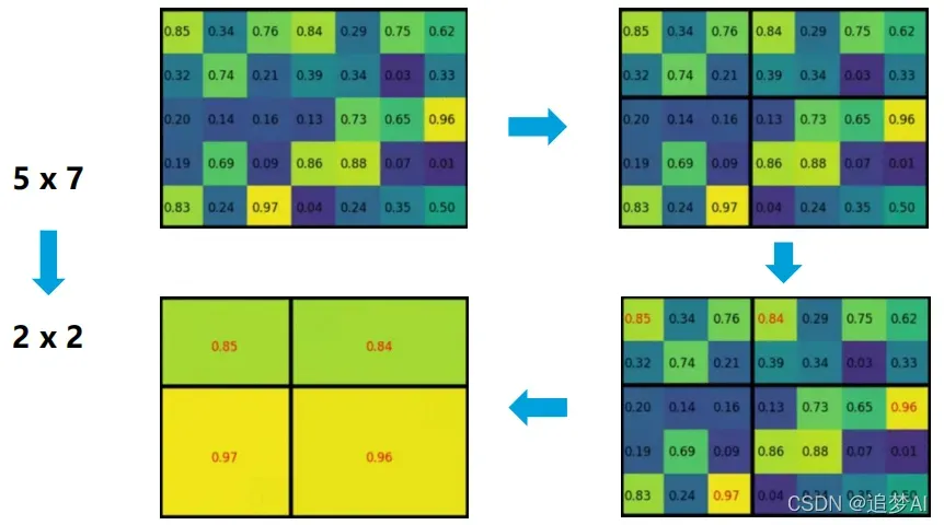
RoIPooling:利用特征采样,把不同空间大小的特征,变成空间大小一致的特征。
将图像中ROI区域对应到卷积特征图中,将这个对应后的卷积特征区域通过池化操作固定到特定大小的特征,然后将特征送入全连接层。
为什么要使用RoIPooling把不同大小的特征变成固定大小?
① 网络后面是全连接层( FC层),要求输入有固定的维度;
② 各个候选区域的特征大小一致,可以组成batch进行处理。
三、Faster R-CNN
大家应该记得,在上述两种算法当中,虽说速度有了很大的提升,但其实还有一个速度慢的地方没有解决,那就是通过Selective Search算法生成候选区域的过程。那么在Faster R-CNN中是如何解决的呢?
下面我们来具体看看。
首先我们先来了解一个概念。Anchors,什么是Anchors?
如图:
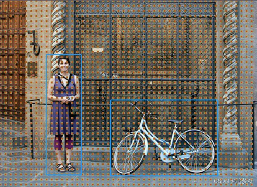
假设这是一张MN大小的图像,那么我们可以认为是为MN个像素点组成的,那么Anchors就是我们人为在这些图像像素点上根据一定的比例设置的一种框。
下图为一个像素点所生成的Anchors.
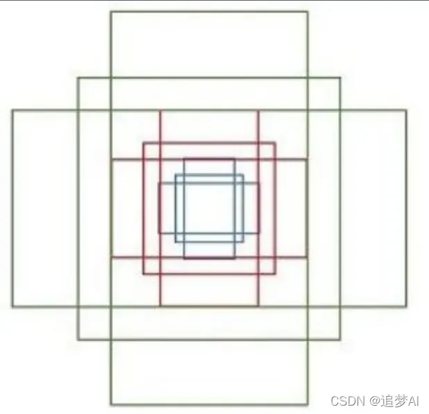
其中一些参数如下:
每个矩形分别有4个值(x1,y1,x2,y2),分别为左上角,右下角的坐标。
九个矩形共有三种形状,长宽比大约为{1:1,1:2,2:1}
我们为图像上所有像素点都配备九种Anchors作为初始的检测层。
Anchors的计算:
假设原图为800600,经过VGG下采样32倍之后,feature map每个点设置9个anchors,所以(800/32)(600/32)9 = 5038*9 = 17100个。
生成的Anchors代码如下:
def generate_anchor_base(base_size=16,
                         ratios=[0.5, 1, 2],
                         anchor_scales=[8, 16, 32]):
    """默认生成左上角9个anchor_base"""
    py = base_size / 2.
    px = base_size / 2.

    anchor_base = np.zeros((len(ratios) * len(anchor_scales), 4),
                           dtype=np.float32)
    for i in range(len(ratios)):
        for j in range(len(anchor_scales)):
            # 生成9种不同比例的h和w
            h = base_size * anchor_scales[j] * np.sqrt(ratios[i])
            w = base_size * anchor_scales[j] * np.sqrt(1. / ratios[i])

            index = i * len(anchor_scales) + j
            # 计算出anchor_base画的9个框的左下角和右上角的4个anchor坐标值
            anchor_base[index, 0] = py - h / 2.
            anchor_base[index, 1] = px - w / 2.
            anchor_base[index, 2] = py + h / 2.
            anchor_base[index, 3] = px + w / 2.
    return anchor_base
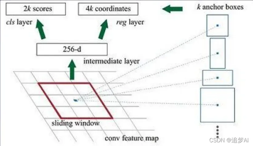
原文中使用的是ZF model中,其 Conv Layers中最后的conv5层 num_output=256,对应生成256 张特征图,所以相当于feature map每个点都是256-dimensions
训练程序会在合适的anchors中随机 选取128个postive anchors+128 个negative anchors进行训练
代码如下所示:
class ProposalTargetCreator(object):
    # 为2000个rois赋予ground truth!(严格讲挑出128个赋予ground truth!)
    # 输入:2000个rois、一个batch(一张图)中所有的bbox ground truth(R,4)、对应bbox所包含的label(R,1)(VOC2007来说20类0-19)
    # 输出:128个sample roi(128,4)、128个gt_roi_loc(128,4)、128个gt_roi_label(128,1)

    def __init__(self,
                 n_sample=128,
                 pos_ratio=0.25, pos_iou_thresh=0.5,
                 neg_iou_thresh_hi=0.5, neg_iou_thresh_lo=0.0
                 ):
        self.n_sample = n_sample
        self.pos_ratio = pos_ratio
        self.pos_iou_thresh = pos_iou_thresh
        self.neg_iou_thresh_hi = neg_iou_thresh_hi
        self.neg_iou_thresh_lo = neg_iou_thresh_lo  # NOTE:default 0.1 in py-faster-rcnn

    def __call__(self, roi, bbox, label,
                 loc_normalize_mean=(0., 0., 0., 0.),
                 loc_normalize_std=(0.1, 0.1, 0.2, 0.2)):
        # 因为这些数据是要放入到整个大网络里进行训练的,比如说位置数据,所以要对其位置坐标进行数据增强处理(归一化处理)
        n_bbox, _ = bbox.shape
        n_bbox, _ = bbox.shape

        roi = np.concatenate((roi, bbox), axis=0)  # 首先将2000个roi和m个bbox给concatenate了一下成为新的roi(2000+m,4)。
        # n_sample = 128,pos_ratio=0.5,round 对传入的数据进行四舍五入
        pos_roi_per_image = np.round(self.n_sample * self.pos_ratio)
        iou = bbox_iou(roi, bbox) #计算每一个roi与每一个bbox的iou
        # 按行找到最大值,返回最大值对应的序号以及其真正的IOU。
        gt_assignment = iou.argmax(axis=1)
        max_iou = iou.max(axis=1)  # 每个roi与对应bbox最大的iou
        # Offset range of classes from [0, n_fg_class - 1] to [1, n_fg_class].
        #  0 是背景.
        gt_roi_label = label[gt_assignment] + 1  # 从1开始的类别序号,给每个类得到真正的label(将0-19变为1-20)

        # 根据iou的最大值将正负样本找出来,pos_iou_thresh=0.5
        pos_index = np.where(max_iou >= self.pos_iou_thresh)[0]
        # 需要保留的roi个数(满足大于pos_iou_thresh条件的roi与64之间较小的一个)
        pos_roi_per_this_image = int(min(pos_roi_per_image, pos_index.size))
        if pos_index.size > 0:
            pos_index = np.random.choice(
                pos_index, size=pos_roi_per_this_image, replace=False)  # 找出的样本数目过多就随机丢掉一些


        # 负样本的ROI区间 [neg_iou_thresh_lo, neg_iou_thresh_hi)
        # neg_iou_thresh_hi=0.5,neg_iou_thresh_lo=0.0
        neg_index = np.where((max_iou < self.neg_iou_thresh_hi) &
                             (max_iou >= self.neg_iou_thresh_lo))[0]
        # 需要保留的roi个数(满足大于0小于neg_iou_thresh_hi条件的roi与64之间较小的一个)
        neg_roi_per_this_image = self.n_sample - pos_roi_per_this_image
        neg_roi_per_this_image = int(min(neg_roi_per_this_image,
                                         neg_index.size))
        if neg_index.size > 0:
            neg_index = np.random.choice(
                neg_index, size=neg_roi_per_this_image, replace=False) # 找出的样本数目过多就随机丢掉一些

        # 综合下找到的正负样本的index
        keep_index = np.append(pos_index, neg_index)
        gt_roi_label = gt_roi_label[keep_index]
        gt_roi_label[pos_roi_per_this_image:] = 0  # 负样本label 设为0
        sample_roi = roi[keep_index]

        # 那么此时输出的128*4的sample_roi就可以去扔到 RoIHead网络里去进行分类与回归了。
        # 同样, RoIHead网络利用这sample_roi+featue为输入,输出是分类(21类)和回归(进一步微调bbox)的预测值,
        # 那么分类回归的groud truth就是ProposalTargetCreator输出的gt_roi_label和gt_roi_loc。
        gt_roi_loc = bbox2loc(sample_roi, bbox[gt_assignment[keep_index]])
        gt_roi_loc = ((gt_roi_loc - np.array(loc_normalize_mean, np.float32)
                       ) / np.array(loc_normalize_std, np.float32))
        # ProposalTargetCreator首次用到了真实的21个类的label,且该类最后对loc进行了归一化处理,所以预测时要进行均值方差处理

        return sample_roi, gt_roi_loc, gt_roi_label
用于生成训练Anchors的代码,可以在开头github代码中找到,有需要的可以理解一下:
class AnchorTargetCreator(object):
# 作用是生成训练要用的anchor(与对应框iou值最大或者最小的各128个框的坐标和256个label(0或者1))
# 为Faster-RCNN专有的RPN网络提供自我训练的样本,RPN网络正是利用AnchorTargetCreator产生的样本作为数据进行网络的训练和学习的,
# 这样产生的预测anchor的类别和位置才更加精确,anchor变成真正的ROIS需要进行位置修正,
# 而AnchorTargetCreator产生的带标签的样本就是给RPN网络进行训练学习用哒


    def __init__(self,
                 n_sample=256,
                 pos_iou_thresh=0.7, neg_iou_thresh=0.3,
                 pos_ratio=0.5):
        self.n_sample = n_sample
        self.pos_iou_thresh = pos_iou_thresh
        self.neg_iou_thresh = neg_iou_thresh
        self.pos_ratio = pos_ratio

    def __call__(self, bbox, anchor, img_size):
        """Assign ground truth supervision to sampled subset of anchors.
        Types of input arrays and output arrays are same.
        """

        img_H, img_W = img_size

        n_anchor = len(anchor)  # 一般对应20000个左右anchor
        inside_index = _get_inside_index(anchor, img_H, img_W) # 将那些超出图片范围的anchor全部去掉,只保留位于图片内部的序号
        anchor = anchor[inside_index] # 保留位于图片内部的anchor
        argmax_ious, label = self._create_label(
            inside_index, anchor, bbox) # 筛选出符合条件的正例128个负例128并给它们附上相应的label
        # 计算每一个anchor与对应bbox求得iou最大的bbox计算偏移量(注意这里是位于图片内部的每一个)
        loc = bbox2loc(anchor, bbox[argmax_ious])
        # 将位于图片内部的框的label对应到所有生成的20000个框中(label原本为所有在图片中的框的)
        label = _unmap(label, n_anchor, inside_index, fill=-1)
        # 将回归的框对应到所有生成的20000个框中(label原本为所有在图片中的框的)
        loc = _unmap(loc, n_anchor, inside_index, fill=0)

        return loc, label

    def _create_label(self, inside_index, anchor, bbox):
        # label: 1 is positive, 0 is negative, -1 is dont care
        label = np.empty((len(inside_index),), dtype=np.int32)  #inside_index为所有在图片范围内的anchor序号
        label.fill(-1) #全部填充-1
        # 调用_calc_ious()函数得到每个anchor与哪个bbox的iou最大以及这个iou值、每个bbox与哪个anchor的iou最大
        argmax_ious, max_ious, gt_argmax_ious = \
            self._calc_ious(anchor, bbox, inside_index)

        # 把每个anchor与对应的框求得的iou值与负样本阈值比较,若小于负样本阈值,
        # 则label设为0,pos_iou_thresh=0.7, neg_iou_thresh=0.3
        label[max_ious < self.neg_iou_thresh] = 0

        # 把与每个bbox求得iou值最大的anchor的label设为1
        label[gt_argmax_ious] = 1

        # 把每个anchor与对应的框求得的iou值与正样本阈值比较,若大于正样本阈值,则label设为1
        label[max_ious >= self.pos_iou_thresh] = 1

        # 按照比例计算出正样本数量,pos_ratio=0.5,n_sample=256
        n_pos = int(self.pos_ratio * self.n_sample)
        pos_index = np.where(label == 1)[0]  # 得到所有正样本的索引
        if len(pos_index) > n_pos:
            disable_index = np.random.choice(
                pos_index, size=(len(pos_index) - n_pos), replace=False)
            label[disable_index] = -1  # 如果选取出来的正样本数多于预设定的正样本数,则随机抛弃,将那些抛弃的样本的label设为-1

        # 设定的负样本的数量
        n_neg = self.n_sample - np.sum(label == 1)
        neg_index = np.where(label == 0)[0] #负样本的索引
        if len(neg_index) > n_neg:
            disable_index = np.random.choice(
                neg_index, size=(len(neg_index) - n_neg), replace=False)
            label[disable_index] = -1  # 随机选择不要的负样本,个数为len(neg_index)-neg_index,label值设为-1

        return argmax_ious, label

    def _calc_ious(self, anchor, bbox, inside_index):
        # 调用bbox_iou函数计算anchor与bbox的IOU, ious:(N,K),N为anchor中第N个,K为bbox中第K个,N大概有15000个
        ious = bbox_iou(anchor, bbox)
        argmax_ious = ious.argmax(axis=1)
        # 求出每个anchor与哪个bbox的iou最大,以及最大值,max_ious:[1,N]
        max_ious = ious[np.arange(len(inside_index)), argmax_ious]
        gt_argmax_ious = ious.argmax(axis=0)
        # 求出每个bbox与哪个anchor的iou最大,以及最大值,gt_max_ious:[1,K]
        gt_max_ious = ious[gt_argmax_ious, np.arange(ious.shape[1])]
        gt_argmax_ious = np.where(ious == gt_max_ious)[0]  # 然后返回最大iou的索引(每个bbox与哪个anchor的iou最大),有K个

        return argmax_ious, max_ious, gt_argmax_ious
了解了Anchors机制,下面我们来具体看看Faster R-CNN中的细节。
Faster RCNN的总体流程如下图所示:
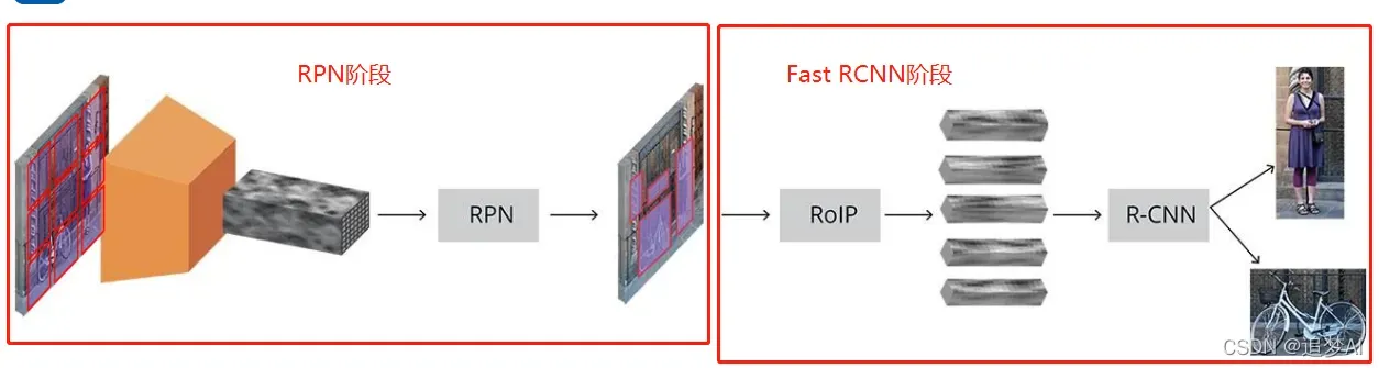
我们广泛的认为:Faster R-CNN = RPN + Fast R-CNN。
RPN阶段
看到这相信大家又会有一个疑惑,什么是RPN?干什么用的?输入输出分别是什么?下面来为大家一一解答。
我们输入一张图像进入到VGG16网络中进行特征提取,得到Feature map,然后再Feature map上铺设我们上述讲的初始Anchors.—>这就是RPN的输入。
那么RPN实际上有两个作用:
①对Anchors做二分类(前景,背景)
②对前景Anchors进行一个微调,把物体尽可能精确的框出来。
注意:我这里用的是尽可能精确!
分类:
由于我们Feature map上的初始Anchors数量过多,所以我们对Anchors进行一个softmax二分类,得到前包含物体的概率和正负例Anchors。
正例:对于每个Anchors与gt box的IOU最大的和所有Anchors与gt box的IOU大于阈值0.7的,我们就认为是一个前景。
负例:小于一定阈值(0.3)的则认为是背景。其他忽略。
回归:
我们的目的是寻找一种关系,对于原始的Anchors经过映射得到一个和gt更接近的窗口。
Anchor box与predicted box, ground truth之间的平移量关系如下:
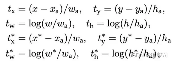
其中xa,ya表示Anchor box中心点的位置,wa,ha则表示宽高。
x,y表示predicted box中心点的位置,w,h则表示宽高。
所以上面两行公式建立的是Anchor box与predicted box的关系,predicted box就是RPN得到的结果。
x*,y表示gt中心点的位置,w,h*则表示宽高。
后两行建立的是predicted box, ground truth之间的关系,我们通过RPN得出的结果与gt进行拟合,使得这两个框重合度越来越高。
综上所述:
RPN目的:判定哪些anchors有可能包含物体
输入:所有的anchors
输出:(1)包含物体的概率
(2)调整anchors的位置
RPN代码如下:
class RegionProposalNetwork(nn.Module):
    """
        1.计算回归坐标偏移量
        2.计算anchors前景概率
        3.调用ProposalCreator和使用NMS得出2000个近似目标框的坐标
    """


    def __init__(self,
                 in_channels=512,
                 mid_channels=512,
                 ratios=[0.5, 1, 2],
                 anchor_scales=[8, 16, 32],
                 feat_stride=16,
                 proposal_creator_params=dict()):

        super(RegionProposalNetwork, self).__init__()
        # 调用 generate_anchor_base()函数,生成左上角9个anchor_base
        self.anchor_base = generate_anchor_base(
            anchor_scales=anchor_scales, ratios=ratios)
        self.feat_stride = feat_stride
        self.proposal_layer = ProposalCreator(self, **proposal_creator_params)  # 输出2000roi
        n_anchor = self.anchor_base.shape[0]  # 9个
        self.conv1 = nn.Conv2d(in_channels, mid_channels, 3, 1, 1)
        self.score = nn.Conv2d(mid_channels, n_anchor * 2, 1, 1, 0)
        self.loc = nn.Conv2d(mid_channels, n_anchor * 4, 1, 1, 0)
        #作归一化处理
        normal_init(self.conv1, 0, 0.01)
        normal_init(self.score, 0, 0.01)
        normal_init(self.loc, 0, 0.01)

    def forward(self, x, img_size, scale=1.):
        """Forward Region Proposal Network.

        """
        n, _, hh, ww = x.shape  # (batch_size,512,H/16,W/16),其中H,W分别为原图的高和宽
        anchor = _enumerate_shifted_anchor(
            np.array(self.anchor_base),
            self.feat_stride, hh, ww)  # 在9个base_anchor基础上生成hh*ww*9个anchor,对应到原图坐标

        n_anchor = anchor.shape[0] // (hh * ww)  # hh*ww*9/hh*ww=9
        h = F.relu(self.conv1(x)) # 512个3x3卷积(512, H/16,W/16)

        rpn_locs = self.loc(h)  # n_anchor(9)*4个1x1卷积,回归坐标偏移量。(9*4,hh,ww)

        # 转换为(n,hh,ww,9*4)后变为(n,hh*ww*9,4)
        rpn_locs = rpn_locs.permute(0, 2, 3, 1).contiguous().view(n, -1, 4)
        rpn_scores = self.score(h)  # n_anchor(9)*2个1x1卷积,回归类别。(9*2,hh,ww)
        rpn_scores = rpn_scores.permute(0, 2, 3, 1).contiguous()  # 转换为(n,hh,ww,9*2)
        rpn_softmax_scores = F.softmax(rpn_scores.view(n, hh, ww, n_anchor, 2), dim=4)  # 计算softmax
        rpn_fg_scores = rpn_softmax_scores[:, :, :, :, 1].contiguous()  # 得到前景的分类概率
        rpn_fg_scores = rpn_fg_scores.view(n, -1)  # 得到所有anchor的前景分类概率
        rpn_scores = rpn_scores.view(n, -1, 2)  # 得到每一张feature map上所有anchor的网络输出值

        rois = list()
        roi_indices = list()
        for i in range(n):  # n为batch_size数

        # 调用ProposalCreator函数, rpn_locs维度(hh*ww*9,4),rpn_fg_scores维度为(hh*ww*9),
        # anchor的维度为(hh*ww*9,4), img_size的维度为(3,H,W),H和W是经过数据预处理后的。
        # 计算(H/16)x(W/16)x9(大概20000)个anchor属于前景的概率,取前12000个并经过NMS得到2000个近似目标框的坐标。
            roi = self.proposal_layer(
                rpn_locs[i].cpu().data.numpy(), #位置信息
                rpn_fg_scores[i].cpu().data.numpy(), #前景概率
                anchor, img_size,
                scale=scale)
            batch_index = i * np.ones((len(roi),), dtype=np.int32)
            rois.append(roi)
            roi_indices.append(batch_index)

        rois = np.concatenate(rois, axis=0) # rois为所有batch_size的roi
        roi_indices = np.concatenate(roi_indices, axis=0)  # 按行拼接
        # rpn_locs的维度(hh*ww*9,4),rpn_scores维度为(hh*ww*9,2),
        # rois的维度为(2000,4),roi_indices用不到,anchor的维度为(hh*ww*9,4)
        return rpn_locs, rpn_scores, rois, roi_indices, anchor


def _enumerate_shifted_anchor(anchor_base, feat_stride, height, width):
    # 在整个特征图生成所有的anchor,对应回原图大小

    import numpy as xp
    shift_y = xp.arange(0, height * feat_stride, feat_stride)  # 纵向偏移量(0,16,32,...)
    shift_x = xp.arange(0, width * feat_stride, feat_stride)  # 横向偏移量(0,16,32,...)
    # shift_x = [[0,16,32,..],[0,16,32,..], [0,16,32,..]...],
    # shift_y = [[0,0,0,..],[16,16,16,..], [32,32,32,..]...],
    # 就是形成了一个纵横向偏移量的矩阵,也就是特征图的每一点都能够通过这个矩阵找到映射在原图中的具体位置!
    shift_x, shift_y = xp.meshgrid(shift_x, shift_y)
    # 产生偏移坐标对,一个朝x方向,一个朝y方向偏移。
    shift = xp.stack((shift_y.ravel(), shift_x.ravel(),
                      shift_y.ravel(), shift_x.ravel()), axis=1)

    A = anchor_base.shape[0] # A=9
    K = shift.shape[0]  # 读取特征图中元素的总个数
    #用基础的9个anchor的坐标分别和偏移量相加,最后得出了所有的anchor的坐标,
    # 四列可以堪称是左上角的坐标和右下角的坐标加偏移量的同步执行,飞速的从
    # 上往下捋一遍,所有的anchor就都出来了!一共K个特征点,每一个有A(9)个
    # 基本的anchor,所以最后reshape((K*A),4)的形式,也就得到了最后的所有
    # 的anchor左下角和右上角坐标.
    anchor = anchor_base.reshape((1, A, 4)) + \
             shift.reshape((1, K, 4)).transpose((1, 0, 2))  # (k, 1, 4)
    # np 的广播机制 anchor.shape =(k,A,4)
    anchor = anchor.reshape((K * A, 4)).astype(np.float32)
    return anchor


def _enumerate_shifted_anchor_torch(anchor_base, feat_stride, height, width):
    # Enumerate all shifted anchors:
    #
    # add A anchors (1, A, 4) to
    # cell K shifts (K, 1, 4) to get
    # shift anchors (K, A, 4)
    # reshape to (K*A, 4) shifted anchors
    # return (K*A, 4)

    # !TODO: add support for torch.CudaTensor
    # xp = cuda.get_array_module(anchor_base)
    import torch as t
    shift_y = t.arange(0, height * feat_stride, feat_stride)
    shift_x = t.arange(0, width * feat_stride, feat_stride)
    shift_x, shift_y = xp.meshgrid(shift_x, shift_y)
    shift = xp.stack((shift_y.ravel(), shift_x.ravel(),
                      shift_y.ravel(), shift_x.ravel()), axis=1)

    A = anchor_base.shape[0]
    K = shift.shape[0]
    anchor = anchor_base.reshape((1, A, 4)) + \
             shift.reshape((1, K, 4)).transpose((1, 0, 2))
    anchor = anchor.reshape((K * A, 4)).astype(np.float32)
    return anchor


def normal_init(m, mean, stddev, truncated=False):
    """
    weight initalizer: truncated normal and random normal.
    """
    # x is a parameter
    if truncated:
        m.weight.data.normal_().fmod_(2).mul_(stddev).add_(mean)  # not a perfect approximation
    else:
        m.weight.data.normal_(mean, stddev)
        m.bias.data.zero_()
Fast RCNN阶段
我们再来看看Faster RCNN的整体网络结构图:
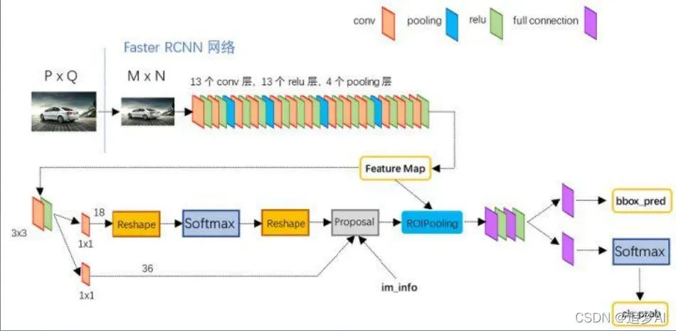
通过网络结构可知RPN和ROIPooling是共享卷积层的。
以VGG网络为例:Conv layers部分共有13个conv层, 13个relu层,4个pooling层。
• 所有的conv层都是:kernel_size=3,pad=1, stride=1
• 所有的pooling层都是:kernel_size=2,pad=0, stride=2
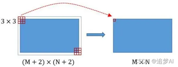
• 在Faster RCNN Conv layers中对所有的卷积都做了扩边处理( pad=1,即填充一圈0),导致原图变为 (M+2)x(N+2)大小,再做3×3卷积后输出MxN 。
• pooling层kernel_size=2,stride=2。这样每个经过 pooling层的MxN矩阵,都会变为(M/2)x(N/2)大小。
• 一个MxN大小的矩阵经过Conv layers固定变为 (M/16)x(N/16)
直到ROIPooling之前,VGG输出50x38x512, 对应50x38xk个anchors
• RPN输出: 50x38x2k的正例/负例 (2k是因为有正负例)
50x38x4k的regression坐标回归特征矩阵(4k是因为每个anchors都有4个位置信息)
图中有个proposal层,Proposal Layer负责综合变换量和正例anchors, 计算出精准的proposal。
3个输入: anchors分类结果,对应bbox的变换量和缩放信息
什么是缩放信息?
缩放信息:若经过4次pooling后WxH=(M/16)x(N/16),则缩放量为16
具体流程如下:
① 生成anchors,依据变换量对所有的anchors做bbox regression回归。
② 按照输入的正例 softmax scores由大到小排序anchors,提取前pre_nms_topN(e.g. 6000)个anchors。
③ 限定超出图像边界的positive anchors为图像边界,防止后续roi pooling时proposal超出图像边界
④ 剔除尺寸非常小的positive anchors。
⑤ 对剩余的positive anchors进行NMS。
⑥ 之后输出proposal=[x1, y1, x2, y2],对应的是MxN的图像尺度。
后续的ROIPooling信息:
由图可知:
两个输入 ① 原始的feature maps ② RPN输出的proposal boxes
注意:此时的proposal boxes是对应M*N的尺度。即原图尺度。
proposals代码如下:
class ProposalCreator:

    """
    这部分的操作不需要进行反向传播,因此可以利用numpy/tensor实现
    对于每张图片,利用它的feature map,计算(H/16)x(W/16)x9(大概20000)个anchor属于前景的概率,
    然后从中选取概率较大的12000张,利用位置回归参数,修正这12000个anchor的位置,
    利用非极大值抑制,选出2000个ROIS以及对应的位置参数。
    """

    def __init__(self,
                 parent_model,
                 nms_thresh=0.7,
                 n_train_pre_nms=12000,
                 n_train_post_nms=2000,
                 n_test_pre_nms=6000,
                 n_test_post_nms=300,
                 min_size=16
                 ):
        self.parent_model = parent_model
        self.nms_thresh = nms_thresh
        self.n_train_pre_nms = n_train_pre_nms
        self.n_train_post_nms = n_train_post_nms
        self.n_test_pre_nms = n_test_pre_nms
        self.n_test_post_nms = n_test_post_nms
        self.min_size = min_size

    def __call__(self, loc, score,
                 anchor, img_size, scale=1.):
        #这里的loc和score是经过region_proposal_network中经过1x1卷积分类和回归得到的
        if self.parent_model.training:
            n_pre_nms = self.n_train_pre_nms   #NMS之前有12000个
            n_post_nms = self.n_train_post_nms #经过NMS后有2000个
        else:
            n_pre_nms = self.n_test_pre_nms    #6000->300
            n_post_nms = self.n_test_post_nms


        # 把anchors转成proposal,即rois
        roi = loc2bbox(anchor, loc)

        # Clip predicted boxes to image.
        roi[:, slice(0, 4, 2)] = np.clip(
            roi[:, slice(0, 4, 2)], 0, img_size[0])#裁剪将rois的ymin,ymax限定在[0,H]
        roi[:, slice(1, 4, 2)] = np.clip(
            roi[:, slice(1, 4, 2)], 0, img_size[1])#裁剪将rois的xmin,xmax限定在[0,W]


        #去除太小的预测框
        min_size = self.min_size * scale #16
        hs = roi[:, 2] - roi[:, 0] #rois的宽
        ws = roi[:, 3] - roi[:, 1] #rois的长
        keep = np.where((hs >= min_size) & (ws >= min_size))[0] #确保rois的长宽大于最小阈值
        roi = roi[keep, :]
        score = score[keep] #对剩下的ROIs进行打分(根据region_proposal_network中rois的预测前景概率)

        # 对所有的(proposal, score)按打分从大到小排列
        #选择最前面 pre_nms_topN (e.g. 6000)个
        order = score.ravel().argsort()[::-1]
        if n_pre_nms > 0:
            order = order[:n_pre_nms]
        roi = roi[order, :]
        score = score[order]


        #使用NMS,选择after_nms_topN (e.g. 300)个.
        keep = nms(
            torch.from_numpy(roi).cuda(),
            torch.from_numpy(score).cuda(),
            self.nms_thresh)
        if n_post_nms > 0:
            keep = keep[:n_post_nms]
        roi = roi[keep.cpu().numpy()]
        return roi
在本文开头已经介绍了ROIPooling的原理。下面来说说这个的具体步骤与作用。
为什么要用ROIPooling?
因为proposals大小形状各不相同
由于这里的feature maps是对应(M/16)(N/16)大小的,所以这里我们要把proposals大小给对应成(M/16)(N/16)大小。
再将每个proposals对应的feature maps部分分成wh个网格。对每一个网格的每一份都做maxpooling处理。
这样处理过后,即使大小不同的proposal输出结果都是wh固定大小。
然后:
① 通过全连接和softmax对proposals进行分类
② 再次对proposals进行bounding box regression,获 取更高精度的bbox。
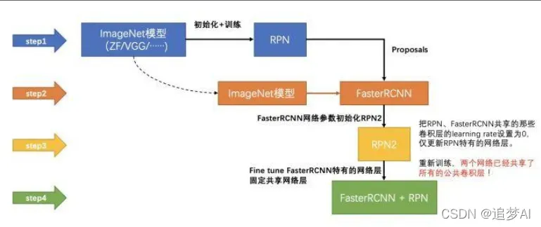
Faster RCNN的训练
① 训练RPN,该网络用ImageNet预训练的模型 初始化;
② 我们利用第一步的RPN生成的建议框,由 Fast R-CNN训练一个单独的检测网络这个检测网络同样是由ImageNet预训练的模型 初始化的;
③ 我们用检测网络初始化RPN训练,但我们固 定共享的卷积层,并且只微调RPN独有的层,现在两个网络共享卷积层了;
④ 保持共享的卷积层固定,微调Fast R-CNN的 fc层。这样,两个网络共享相同的卷积层, 构成一个统一的网络。
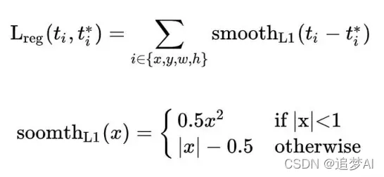
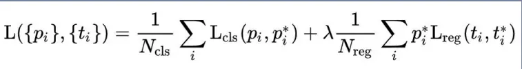
总体的loss计算比较简单,这里不详细讲。公式如下:

① cls class:用于分类网络训练。采用的是log loss。
其他训练方式:
1.Approximate joint training: u RPN和Fast R-CNN合为一个网络
前向传播时, proposal由RPN层输出
反向传播时,共享层的传播误差等于RPN loss和Fast R-CNN loss之和
注意这种方法里proposal的坐标预测的梯度被忽略
能够缩减25-50%的训练时间
2 . Non-approximate joint training:不舍弃proposal 的坐标预测梯度
网络总结
step_0: 基于ZF或VGG16提取输入图像特征
step_1: 生成anchors
step_2: RPN计算:特征图feature map通过RPN预测anchor参数:置信度 (foreground)和转为预测框的坐标系数
step_3: 根据anchors和RPN预测的anchors参数,计算预测框的坐标系数, 并得到每个预测框的所属类别labels。
step_4: ROI Pooling把目标转为统一的固定尺寸。
step_5: Fast RCNN 预测预测框的类别,和转为目标框的平移缩放系数。注 意:这里要与RPN区分
Faster RCNN网络代码如下:
def decom_vgg16():
    # the 30th layer of features is relu of conv5_3
    if opt.caffe_pretrain: #是否使用caffe预训练
        model = vgg16(pretrained=False)
        if not opt.load_path:
            model.load_state_dict(t.load(opt.caffe_pretrain_path))
    else:
        model = vgg16(not opt.load_path)

    features = list(model.features)[:30] #加载预训练模型vgg16的conv5_3之前的部分
    classifier = model.classifier

    classifier = list(classifier)
    del classifier[6] #删除最后分1000类
    if not opt.use_drop: #删除两个dropout
        del classifier[5]
        del classifier[2]
    classifier = nn.Sequential(*classifier)

    for layer in features[:10]: #冻结vgg16前2个stage,不进行反向传播
        for p in layer.parameters():
            p.requires_grad = False

    return nn.Sequential(*features), classifier #拆分为特征提取网络和分类网络


class FasterRCNNVGG16(FasterRCNN):
    """Faster R-CNN based on VGG-16."""
    #分别对特征VGG16的特征提取部分、分类部分、RPN网络、VGG16RoIHead网络进行了实例化
    feat_stride = 16  # downsample 16x for output of conv5 in vgg16

    def __init__(self,
                 n_fg_class=20,
                 ratios=[0.5, 1, 2],
                 anchor_scales=[8, 16, 32]
                 ): #总类别数为20类,三种尺度三种比例的anchor

        extractor, classifier = decom_vgg16() #conv5_3及之前的部分,分类器

        rpn = RegionProposalNetwork(
            512, 512,
            ratios=ratios,
            anchor_scales=anchor_scales,
            feat_stride=self.feat_stride,
        ) #返回rpn_locs, rpn_scores, rois, roi_indices, anchor

        head = VGG16RoIHead(
            n_class=n_fg_class + 1,
            roi_size=7,
            spatial_scale=(1. / self.feat_stride),
            classifier=classifier
        ) #下面会分析VGG16RoIHead(),n_class = 21(加上背景)

        super(FasterRCNNVGG16, self).__init__(
            extractor,
            rpn,
            head,
        ) #相当于给faster_rcnn传入参数extractor, rpn, head


class VGG16RoIHead(nn.Module):
    """Faster R-CNN Head for VGG-16 based implementation.
    This class is used as a head for Faster R-CNN.
    This outputs class-wise localizations and classification based on feature
    maps in the given RoIs.
    """

    def __init__(self, n_class, roi_size, spatial_scale,
                 classifier):
        # n_class includes the background
        super(VGG16RoIHead, self).__init__()

        self.classifier = classifier #vgg16中的classifier
        self.cls_loc = nn.Linear(4096, n_class * 4)
        self.score = nn.Linear(4096, n_class)

        normal_init(self.cls_loc, 0, 0.001)
        normal_init(self.score, 0, 0.01) #全连接层权重初始化

        self.n_class = n_class #加上背景21类
        self.roi_size = roi_size #7
        self.spatial_scale = spatial_scale # 1/16
        #将大小不同的roi变成大小一致,得到pooling后的特征,大小为[300, 512, 7, 7]。.利用Cupy实现在线编译的
        #使用的是from torchvision.ops import RoIPool
        self.roi = RoIPool( (self.roi_size, self.roi_size),self.spatial_scale)
    def forward(self, x, rois, roi_indices):
        """Forward the chain."""
        # in case roi_indices is  ndarray
        roi_indices = at.totensor(roi_indices).float() #ndarray->tensor
        rois = at.totensor(rois).float()
        indices_and_rois = t.cat([roi_indices[:, None], rois], dim=1)
        # NOTE: important: yx->xy
        xy_indices_and_rois = indices_and_rois[:, [0, 2, 1, 4, 3]]
        indices_and_rois =  xy_indices_and_rois.contiguous() #把tensor变成在内存中连续分布的形式

        pool = self.roi(x, indices_and_rois) #ROIPOOLING
        pool = pool.view(pool.size(0), -1)
        fc7 = self.classifier(pool) #decom_vgg16()得到的calssifier,得到4096
        roi_cls_locs = self.cls_loc(fc7) #(4096->84) 84=21*4
        roi_scores = self.score(fc7) #(4096->21)
        return roi_cls_locs, roi_scores


def normal_init(m, mean, stddev, truncated=False):
    """
    weight initalizer: truncated normal and random normal.
    """
    # x is a parameter
    if truncated:
        m.weight.data.normal_().fmod_(2).mul_(stddev).add_(mean)  # not a perfect approximation
    else:
        m.weight.data.normal_(mean, stddev)
        m.bias.data.zero_()
训练代码比较简单,这里不做解析,有需要的可以自己尝试配置。
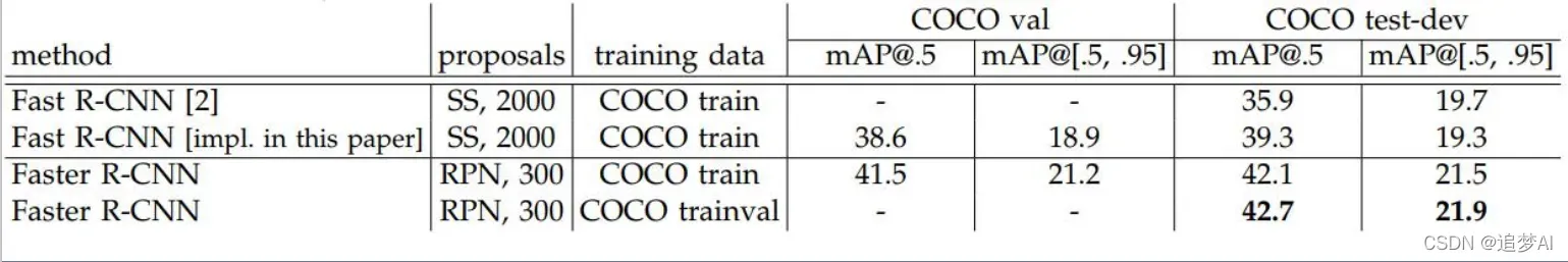
实验结果和分析
和ss对比(PASCAL VOC2007)
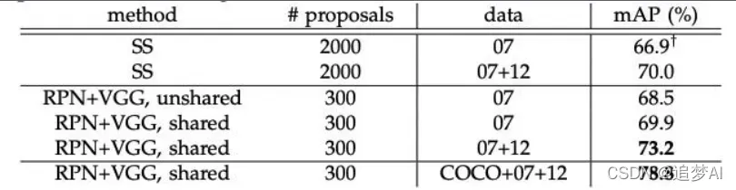
Test on PASCAL VOC 2007
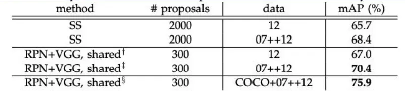
Test on PASCAL VOC 2012
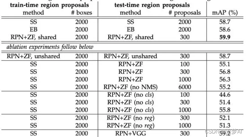
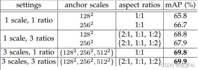
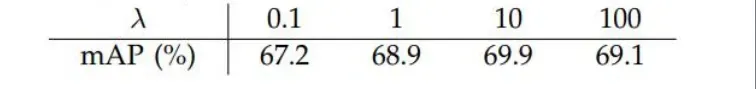
RPN消融实验,PASCAL VOC 2007
文章出处登录后可见!