周志华《机器学习》第三章课后习题

目录

3.1 试析在什么情形下式(3.2) 中不必考虑偏置项 b.

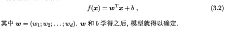
①b与输入毫无关系，如果没有b，y‘=wx必须经过原点
②当两个线性模型相减时，消除了b。可用训练集中每个样本都减去第一个样本，然后对新的样本做线性回归，不用考虑偏置项b。

3.2、试证明，对于参数w,对率回归的目标函数(3.18)是非凸的,但其对数似然函数(3.27)是凸的.

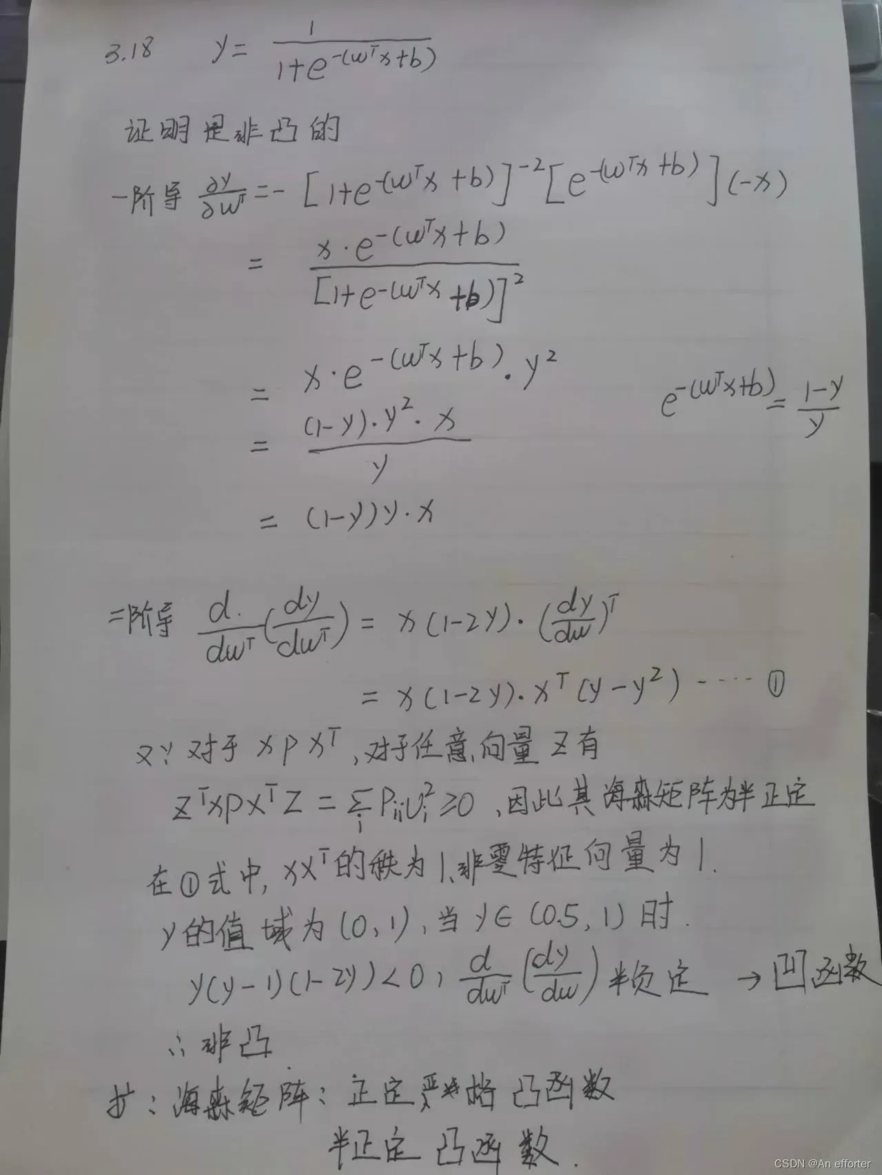
 3.27

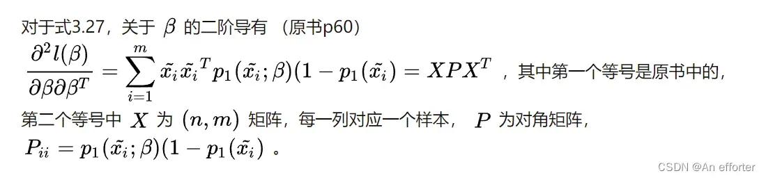
 3.3、编程实现对率回归,并给出西瓜数据集3.0α上的结果.

数据集：

3.3.py

# -*- coding: utf-8 -*

'''
data importion
'''
import numpy as np  # for matrix calculation
import matplotlib.pyplot as plt

# load the CSV file as a numpy matrix
# 将CSV文件加载为numpy矩阵
dataset = np.loadtxt('watermelon3_0_Ch.csv', delimiter=",")

# separate the data from the target attributes
# 将数据与目标属性分离
X = dataset[:, 1:3]
y = dataset[:, 3]

m, n = np.shape(X)

# draw scatter diagram to show the raw data
#绘制出数据点
f1 = plt.figure(1)
plt.title('watermelon_3a')
plt.xlabel('density')
plt.ylabel('ratio_sugar')
plt.scatter(X[y == 0, 0], X[y == 0, 1], marker='o', color='k', s=100, label='bad')
plt.scatter(X[y == 1, 0], X[y == 1, 1], marker='o', color='g', s=100, label='good')
plt.legend(loc='upper right')
# plt.show()

''' 
using sklearn lib for logistic regression
使用sklearn库进行逻辑回归
'''
from sklearn import metrics
from sklearn import model_selection
from sklearn.linear_model import LogisticRegression
import matplotlib.pylab as pl

# generalization of test and train set
# 先划分训练集和测试集，采用sklearn.model_selection.train_test_split()实现
X_train, X_test, y_train, y_test = model_selection.train_test_split(X, y, test_size=0.5, random_state=0)

# model training
# 采用sklearn.linear_model.LogisticRegression，基于训练集直接拟合出逻辑回归模型，然后在测试集上评估模型（查看混淆矩阵和F1值）

log_model = LogisticRegression()  # using log-regression lib model
log_model.fit(X_train, y_train)  # fitting

# model validation 模型确认
y_pred = log_model.predict(X_test)

# summarize the fit of the model  总结模型的拟合情况
print(metrics.confusion_matrix(y_test, y_pred))
print(metrics.classification_report(y_test, y_pred))

precision, recall, thresholds = metrics.precision_recall_curve(y_test, y_pred)

# show decision boundary in plt  在PLT中显示决策边界
# X - some data in 2dimensional np.array   X -二维np.array中的一些数据
f2 = plt.figure(2)
h = 0.001
x0_min, x0_max = X[:, 0].min() - 0.1, X[:, 0].max() + 0.1
x1_min, x1_max = X[:, 1].min() - 0.1, X[:, 1].max() + 0.1
x0, x1 = np.meshgrid(np.arange(x0_min, x0_max, h),
                     np.arange(x1_min, x1_max, h))

# here "model" is your model's prediction (classification) function
# 这里的“模型”是模型的预测(分类)函数
z = log_model.predict(np.c_[x0.ravel(), x1.ravel()])

# Put the result into a color plot 把结果放入颜色图中
z = z.reshape(x0.shape)
# 采用matplotlib.contourf绘制的决策区域和边界，可以看出对率回归分类器还是成功的分出了绝大多数类：
plt.contourf(x0, x1, z, cmap=pl.cm.Paired)

# Plot also the training pointsplt.title('watermelon_3a')
plt.title('watermelon_3a')
plt.xlabel('density')
plt.ylabel('ratio_sugar')
plt.scatter(X[y == 0, 0], X[y == 0, 1], marker='o', color='k', s=100, label='bad')
plt.scatter(X[y == 1, 0], X[y == 1, 1], marker='o', color='g', s=100, label='good')
# plt.show()

'''
coding to implement logistic regression
编码以实现逻辑回归
'''
from sklearn import model_selection

import self_def

# X_train, X_test, y_train, y_test
np.ones(n)
m, n = np.shape(X)
X_ex = np.c_[X, np.ones(m)]  # extend the variable matrix to [x, 1]
X_train, X_test, y_train, y_test = model_selection.train_test_split(X_ex, y, test_size=0.5, random_state=0)

# using gradDescent to get the optimal parameter beta = [w, b] in page-59
beta = self_def.gradDscent_2(X_train, y_train)

# prediction, beta mapping to the model
y_pred = self_def.predict(X_test, beta)

m_test = np.shape(X_test)[0]
# calculation of confusion_matrix and prediction accuracy
# #混淆矩阵的计算和预测精度
cfmat = np.zeros((2, 2))
for i in range(m_test):
    if y_pred[i] == y_test[i] == 0:
        cfmat[0, 0] += 1
    elif y_pred[i] == y_test[i] == 1:
        cfmat[1, 1] += 1
    elif y_pred[i] == 0:
        cfmat[1, 0] += 1
    elif y_pred[i] == 1:
        cfmat[0, 1] += 1

print(cfmat)

self_def.py  是 需要调用的函数

import numpy as np


def likelihood_sub(x, y, beta):
    '''
    @param X: one sample variables
    @param y: one sample label
    @param beta: the parameter vector in 3.27
    @return: the sub_log-likelihood of 3.27
    3.27式子的变成对象
    '''
    return -y * np.dot(beta, x.T) + np.math.log(1 + np.math.exp(np.dot(beta, x.T)))


def likelihood(X, y, beta):
    '''
    @param X: the sample variables matrix
    @param y: the sample label matrix
    @param beta: the parameter vector in 3.27
    @return: the log-likelihood of 3.27
    '''
    sum = 0
    m, n = np.shape(X)

    for i in range(m):
        sum += likelihood_sub(X[i], y[i], beta)

    return sum


def partial_derivative(X, y, beta):  # refer to 3.30 on book page 60  请参阅第60页的3.30
    '''
    @param X: the sample variables matrix
    @param y: the sample label matrix
    @param X:样本变量矩阵
     @param y:样本标签矩阵
    @param beta: the parameter vector in 3.27
    @return: the partial derivative of beta [j]
    '''

    m, n = np.shape(X)
    pd = np.zeros(n)

    for i in range(m):
        tmp = y[i] - sigmoid(X[i], beta)
        for j in range(n):
            pd[j] += X[i][j] * (tmp)
    return pd


def gradDscent_1(X, y):  # implementation of fundational gradDscent algorithms 基本梯度算法的实现
    '''
    @param X: X is the variable matrix
    @param y: y is the label array
    @return: the best parameter estimate of 3.27
    然后基于训练集（注意x->[x,1]），给出基于3.27似然函数的定步长梯度下降法，降低损失，注意这里的偏梯度实现技巧：
    '''
    import matplotlib.pyplot as plt

    h = 0.1  # step length of iterator  迭代器的步长
    max_times = 500  # give the iterative times limit  给出迭代次数的极限
    m, n = np.shape(X)

    b = np.zeros((n, max_times))  # for show convergence curve of parameter 表示参数的收敛曲线
    beta = np.zeros(n)  # parameter and initial  参数和初始
    delta_beta = np.ones(n) * h
    llh = 0
    llh_temp = 0

    for i in range(max_times):
        beta_temp = beta.copy()

        for j in range(n):
            # for partial derivative  偏导数
            beta[j] += delta_beta[j]
            llh_tmp = likelihood(X, y, beta)
            delta_beta[j] = -h * (llh_tmp - llh) / delta_beta[j]

            b[j, i] = beta[j]

            beta[j] = beta_temp[j]

        beta += delta_beta
        llh = likelihood(X, y, beta)

    t = np.arange(max_times)

    f2 = plt.figure(3)

    p1 = plt.subplot(311)
    p1.plot(t, b[0])
    plt.ylabel('w1')

    p2 = plt.subplot(312)
    p2.plot(t, b[1])
    plt.ylabel('w2')

    p3 = plt.subplot(313)
    p3.plot(t, b[2])
    plt.ylabel('b')

    plt.show()
    return beta
'''
采用随机梯度下降法来优化：上面采用的是全局定步长梯度下降法（称之为批量梯度下降），
这种方法在可能会面临收敛过慢和收敛曲线波动情况的同时，每次迭代需要全局计算，
计算量随数据量增大而急剧增大。所以尝试采用随机梯度下降来改善参数迭代寻优过程。
'''

def gradDscent_2(X, y):  # implementation of stochastic gradDscent algorithms  随机梯度算法的实现
    '''
    @param X: X is the variable matrix
    @param y: y is the label array
    @return: the best parameter estimate of 3.27
    随机梯度下降法的核心思想是增量学习：一次只用一个新样本来更新回归系数，从而形成在线流式处理。

     同时为了加快收敛，采用变步长的策略，h随着迭代次数逐渐减小。
    '''
    import matplotlib.pyplot as plt

    m, n = np.shape(X)
    h = 0.5  # step length of iterator and initial
    beta = np.zeros(n)  # parameter and initial
    delta_beta = np.ones(n) * h
    llh = 0
    llh_temp = 0
    b = np.zeros((n, m))  # for show convergence curve of parameter

    for i in range(m):
        beta_temp = beta.copy()

        for j in range(n):
            # for partial derivative
            h = 0.5 * 1 / (1 + i + j)  # change step length of iterator
            beta[j] += delta_beta[j]

            b[j, i] = beta[j]

            llh_tmp = likelihood_sub(X[i], y[i], beta)
            delta_beta[j] = -h * (llh_tmp - llh) / delta_beta[j]

            beta[j] = beta_temp[j]

        beta += delta_beta
        llh = likelihood_sub(X[i], y[i], beta)

    t = np.arange(m)

    f2 = plt.figure(3)

    p1 = plt.subplot(311)
    p1.plot(t, b[0])
    plt.ylabel('w1')

    p2 = plt.subplot(312)
    p2.plot(t, b[1])
    plt.ylabel('w2')

    p3 = plt.subplot(313)
    p3.plot(t, b[2])
    plt.ylabel('b')

    plt.show()

    return beta

#sigmoid函数
def sigmoid(x, beta):
    '''
    @param x: is the predict variable
    @param beta: is the parameter
    @return: the sigmoid function value
    
    '''
    return 1.0 / (1 + np.math.exp(- np.dot(beta, x.T)))


def predict(X, beta):
    '''
    prediction the class lable using sigmoid  使用sigmoid预测类标签
    @param X: data sample form like [x, 1]   数据样本形式如[x, 1]
    @param beta: the parameter of sigmoid form like [w, b]  形如[w, b]的参数
    @return: the class lable array  类标签数组
    '''
    m, n = np.shape(X)
    y = np.zeros(m)

    for i in range(m):
        if sigmoid(X[i], beta) > 0.5: y[i] = 1;
    return y

    return

3.4 选择两个 UCI 数据集，比较 10 折交叉验证法和留一法所估计出的对率回归的错误率。

参考代码： han1057578619/MachineLearning_Zhouzhihua_ProblemSets

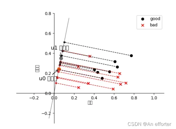
3.5 编辑实现线性判别分析，并给出西瓜数据集 3.0α 上的结果.

 3.5.py

import numpy as np
import pandas as pd
from matplotlib import pyplot as plt


class LDA(object):
    # 绘图，求出均值向量，根据公式3.34和3.39求出类内散度矩阵和类间散度矩阵

    def fit(self, X_, y_, plot_=False):
        pos = y_ == 1
        neg = y_ == 0
        X0 = X_[neg]
        X1 = X_[pos]
        # 均值向量，(1, 2)

        u0 = X0.mean(0, keepdims=True)  # (1, n)
        u1 = X1.mean(0, keepdims=True)

         # 类内散度矩阵，公式3.33，(2, 2)
        sw = np.dot((X0 - u0).T, (X0 - u0)) + np.dot((X1 - u1).T, (X1 - u1))
        # 类间散度矩阵，公式3.37，(1, 2)
        w = np.dot(np.linalg.inv(sw), (u0 - u1).T).reshape(1, -1)

        if plot_:
            fig, ax = plt.subplots()
            ax.spines['right'].set_color('none')
            ax.spines['top'].set_color('none')
            ax.spines['left'].set_position(('data', 0))
            ax.spines['bottom'].set_position(('data', 0))

            plt.scatter(X1[:, 0], X1[:, 1], c='k', marker='o', label='good')
            plt.scatter(X0[:, 0], X0[:, 1], c='r', marker='x', label='bad')

            plt.xlabel('密度', labelpad=1)
            plt.ylabel('含糖量')
            plt.legend(loc='upper right')

            x_tmp = np.linspace(-0.05, 0.15)
            y_tmp = x_tmp * w[0, 1] / w[0, 0]
            plt.plot(x_tmp, y_tmp, '#808080', linewidth=1)

            wu = w / np.linalg.norm(w)

            # 正负样板店
            X0_project = np.dot(X0, np.dot(wu.T, wu))
            plt.scatter(X0_project[:, 0], X0_project[:, 1], c='r', s=15)
            for i in range(X0.shape[0]):
                plt.plot([X0[i, 0], X0_project[i, 0]], [X0[i, 1], X0_project[i, 1]], '--r', linewidth=1)

            X1_project = np.dot(X1, np.dot(wu.T, wu))
            plt.scatter(X1_project[:, 0], X1_project[:, 1], c='k', s=15)
            for i in range(X1.shape[0]):
                plt.plot([X1[i, 0], X1_project[i, 0]], [X1[i, 1], X1_project[i, 1]], '--k', linewidth=1)

            # 中心点的投影
            u0_project = np.dot(u0, np.dot(wu.T, wu))
            plt.scatter(u0_project[:, 0], u0_project[:, 1], c='#FF4500', s=60)
            u1_project = np.dot(u1, np.dot(wu.T, wu))
            plt.scatter(u1_project[:, 0], u1_project[:, 1], c='#696969', s=60)
            # 均值向量的投影点

            ax.annotate(r'u0 投影点',
                        xy=(u0_project[:, 0], u0_project[:, 1]),
                        xytext=(u0_project[:, 0] - 0.2, u0_project[:, 1] - 0.1),
                        size=13,
                        va="center", ha="left",
                        arrowprops=dict(arrowstyle="->",
                                        color="k",
                                        )
                        )

            ax.annotate(r'u1 投影点',
                        xy=(u1_project[:, 0], u1_project[:, 1]),
                        xytext=(u1_project[:, 0] - 0.1, u1_project[:, 1] + 0.1),
                        size=13,
                        va="center", ha="left",
                        arrowprops=dict(arrowstyle="->",
                                        color="k",
                                        )
                        )
            plt.axis("equal")  # 两坐标轴的单位刻度长度保存一致
            plt.show()

        self.w = w
        self.u0 = u0
        self.u1 = u1
        return self

    def predict(self, X):
        project = np.dot(X, self.w.T)

        wu0 = np.dot(self.w, self.u0.T)
        wu1 = np.dot(self.w, self.u1.T)

        return (np.abs(project - wu1) < np.abs(project - wu0)).astype(int)


if __name__ == '__main__':
    data_path = r'watermelon3_0_Ch.csv'

    data = pd.read_csv(data_path).values

    X = data[:, 1:3].astype(float)
    y = data[:, 3]

    y[y == '是'] = 1
    y[y == '否'] = 0
    y = y.astype(int)

    lda = LDA()
    lda.fit(X, y, plot_=True)
    print(lda.predict(X))  # 和逻辑回归的结果一致
    print(y)

想要代码与数据资源的，可以加我微信好友

参考的博客：

(4条消息) 周志华《机器学习》课后习题第三章解答：Ch3.3 – 编程实现对率回归_zhangriqi的博客-CSDN博客

周志华《机器学习》课后习题（第三章）：线性模型-阿里云开发者社区 (aliyun.com)