附:相关需要的工具函数源代码(投影函数、校正矩阵计算等)见最下面
1. 畸变校正
1.1 形成原因
图像畸变一般有两种,第一种是透镜本身的形状有问题,使得图像发生径向畸变;第二种是透镜安装时与成像平面之间不完全平行,导致图像发生切向畸变。畸变会导致图像中物体的形状与实际物体的形状不相同,比如直线变成曲线、矩形拉长等。故而想要得到实际真实图像,必须要根据之前对相机进行标定得到的参数对图像进行畸变的去除。
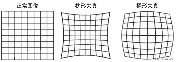
(a)径向畸变
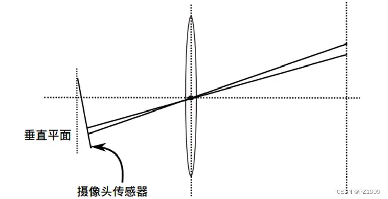
(b)切向畸变
图像畸变示意
1.2 消除办法
畸变去除的基本思路为:
- 假设图像没有发生畸变,将图像由图像坐标系转换到相机坐标系(归一化相机坐标系,即距离为1)
- 根据之前标定好的相机参数,计算畸变之后相机坐标系上的点坐标
- 根据相机内参将畸变之后的相机坐标系上的点坐标变换到图像坐标系下
- 根据计算的点坐标与原始图像进行插值。
具体的原理解析,可以参考文章https://blog.csdn.net/shyjhyp11/article/details/109506149,推导过程非常详细。
function [img_correct,newOrigin] = ImgDistortionCorrection(img,camera,OutputView)
%undistortImage Correct image for lens distortion.
%   [J, newOrigin] = undistortImage(I, intrinsics) removes lens distortion
%   from image I, and returns the result as image J. I can be a grayscale
%   or a truecolor image. intrinsics is either cameraParameters or
%   cameraIntrinsics object.
%
%   newOrigin is a 2-element vector containing the [x,y] location of the
%   origin of the output image J in the intrinsic coordinates of the input
%   image I. Before using extrinsics, pointsToWorld, or triangulate
%   functions you must add newOrigin to the coordinates of points detected
%   in undistorted image J in order to transform them into the intrinsic
%   coordinates of the original image I.
%   If 'OutputView' is set to 'same', then newOrigin is [0, 0].
if OutputView=='same'
    % Para init
    [X,Y] = meshgrid(0:size(img,2)-1,0:size(img,1)-1);
    c_x = camera.center(1,1);
    c_y = camera.center(1,2);
    f_x = camera.focal(1,1);
    f_y = camera.focal(1,2);
    k1 = camera.dis(1,1);
    k2 = camera.dis(1,2);
    g1 = camera.dis(1,3);
    g2 = camera.dis(1,4);
    k3 = camera.dis(1,5);
    % calculate point in camrera coordinate system
    x1 = (X-c_x)/f_x;
    y1 = (Y-c_y)/f_y;
    % calculate dis_point in camrera coordinate system
    r2 = x1.^2+y1.^2;
    x2 = x1.*(1+k1*r2+k2*r2.^2+k3*r2.^3)+2*g1*x1.*y1+g2*(r2+2*x1.^2);
    y2 = y1.*(1+k1*r2+k2*r2.^2+k3*r2.^3)+2*g2*x1.*y1+g1*(r2+2*y1.^2);
    % (u, v) undis (u_d, v_d)
    % calculate dis point in image coordinate system
    u_d = f_x*x2 + c_x+1;
    v_d = f_y*y2 + c_y+1;
    % interp to get undis image
    img_correct = interp2(img, u_d, v_d);
    newOrigin = [0,0];
end
end
注意事项:
(1)与OPENCV结果进行过对比,matlab中的矩阵序号需要减去1以成为坐标,但是仍然存在一定误差,具体原因不明确,希望有大佬给出解释。
2. 极线校正
2.1 基本原因
进行畸变校正获取到真实图像后,为了方便下一步的立体匹配,还需要进行极线校正,即将左右两个相机平面变成一个平面,然后每一行像素相互对应。(下文代码大部分搬运自matlab标定工具箱)
2.2 基本流程
- 计算两个相机平面校正至水平的变换矩阵(但是相机中心以及前后仍存在距离)。
设世界坐标系为左相机坐标系,右相机到左相机的旋转矩阵为R,平移为T,设同一点在左相机为,右相机为
,则可得
。
利用罗德里格斯公式,可将旋转矩阵变换为旋转向量(向量方向
为旋转轴,模
为旋转角度),将旋转角度一份为二,得到
,再反向变换为旋转矩阵
。
则将相机1坐标系旋转,相机2坐标系旋转
,
,可以变换成
。
    % R、T are right camera to left camera,R*C2+T=C1
    % P2=RP1+T
    % Bring the 2 cameras in the same orientation by rotating them "minimally":
    r_r = rodrigues(-camera2.R/2);
    r_l = r_r';
    t = r_r * camera2.T';
- 计算两个平行平面将中心变换到一致的变换矩阵,即将两个坐标系一起进行变换直到基线与X轴平行。(两个坐标系前后一致,且基线与X轴平行)
极线可以视作T,因此计算T到X轴的变换矩阵R2,然后同时对两个坐标系进行变换即可 。
矩阵计算方法:
(1)计算T到X的旋转角度,点乘除以模再计算acos即可。
(2)计算旋转轴,即T与X轴都垂直的方向,叉乘除以两个模即可。
(3)基于罗德里格斯公式计算旋转矩阵。
  % Rotate both cameras so as to bring the translation vector in alignment with the (1;0;0) axis:
    if abs(t(1)) > abs(t(2))
        type_stereo = 0;
        uu = [1;0;0]; % Horizontal epipolar lines
    else
        type_stereo = 1;
        uu = [0;1;0]; % Vertical epipolar lines
    end
    if dot(uu,t)<0
        uu = -uu; % Swtich side of the vector
    end

    % rotate to make the epipolar lines of the two camera images horizontal,the x-axis coincides with t.
    ww = cross(t,uu);
    ww = ww/norm(ww);
    ww = acos(abs(dot(t,uu))/(norm(t)*norm(uu)))*ww; % Rotation angle modulo times the rotation axis
    R2 = rodrigues(ww);
- 虽然相机坐标系已经校正, 但是左右相机内参仍然不同,图像坐标系上仍然不会对齐因此需要对内参进行更改,将左右相机
设置成相同,理论上还有个
,但一般不做考虑。
(1)设置新的内参,将左右相机
   % Computation of the *new* intrinsic parameters for both left and right cameras:
   % Vertical focal length *MUST* be the same for both images (here, we are trying to find a focal length that retains as much information contained in the original distorted images):
   fc_y_new = min(camera1.focal(1,2),camera2.focal(1,2));

   % For simplicity, let's pick the same value for the horizontal focal length as the vertical focal length (resulting into square pixels):
   fc_left_new = round([fc_y_new;fc_y_new]);
   fc_right_new = round([fc_y_new;fc_y_new]);
(2)计算前两步旋转变换之后,如果想将相机坐标系得到的中心点变换到图像坐标系,偏移应该是多少,以确保得到更多图像。首先将原始图像四个角点变换到归一化相机坐标系,然后将其投影到新的图像坐标系(旋转变换后的图像坐标系)下,用理论图像中心点减去四个角点的平均值,即可得到偏移值,为了考虑左右都取较多图像,因此需要取平均值,根据是水平校正还是竖直校正选取平均
。
    % Select the new principal points to maximize the visible area in the rectified images
    % normalize_pixel: Transform the four corners of the original image to the normalized camera plane
    % project_points2:Project the four corners of the normalized plane to the transformed camera coordinate plane, and set new f_x, f_y and c_x, c_y.
    cc_left_new = [(nx-1)/2;(ny-1)/2] - mean(project_points2([normalize_pixel([0  nx-1 nx-1 0; 0 0 ny-1 ny-1],fc_left,cc_left,kc_left,alpha_c_left);[1 1 1 1]],rodrigues(R_L),zeros(3,1),fc_left_new,[0;0],zeros(5,1),0),2);
    cc_right_new = [(nx-1)/2;(ny-1)/2] - mean(project_points2([normalize_pixel([0  nx-1 nx-1 0; 0 0 ny-1 ny-1],fc_right,cc_right,kc_right,alpha_c_right);[1 1 1 1]],rodrigues(R_R),zeros(3,1),fc_right_new,[0;0],zeros(5,1),0),2);
    % For simplivity, set the principal points for both cameras to be the average of the two principal points.
    if ~type_stereo
        %-- Horizontal stereo
        cc_y_new = (cc_left_new(2) + cc_right_new(2))/2;
        cc_left_new = [cc_left_new(1);cc_y_new];
        cc_right_new = [cc_right_new(1);cc_y_new];
    else
        %-- Vertical stereo
        cc_x_new = (cc_left_new(1) + cc_right_new(1))/2;
        cc_left_new = [cc_x_new;cc_left_new(2)];
        cc_right_new = [cc_x_new;cc_right_new(2)];
    end

    % Of course, we do not want any skew or distortion after rectification:
(3)根据最新参数,重新计算图像变换以及插值。
% Pre-compute the necessary indices and blending coefficients to enable quick rectification:
% The original image is changed in the function when Irec_junk_left is calculated, so it cannot be directly used as the corrected image
[Irec_junk_left,ind_new_left,ind_1_left,ind_2_left,ind_3_left,ind_4_left,a1_left,a2_left,a3_ left,a4_left] = rect_index(zeros(ny,nx),R_L,fc_left,cc_left,kc_left,alpha_c_left,KK_left_new);
[Irec_junk_right,ind_new_right,ind_1_right,ind_2_right,ind_3_right,ind_4_right,a1_right,a2_right,a3_right,a4_right] = rect_index(zeros(ny,nx),R_R,fc_right,cc_right,kc_right,alpha_c_right,KK_right_new);

clear Irec_junk_left Irec_junk_right

%图像校正
img_left_rectified = zeros(ny,nx);
img_left_rectified(ind_new_left) = a1_left .* img_left(ind_1_left) + a2_left .* img_left(ind_2_left) + a3_left .* img_left(ind_3_left) + a4_left .* img_left(ind_4_left);
完整函数代码如如下
function [img_left_rectified, img_right_rectified,Q,R1] = PolarlineCorrection(img_left, ...
    img_right, camera1,camera2,flag,alpha,type_stereo)
% rectifyStereoImages Rectifies a pair of stereo images.
%   [img_left_rectified, img_left_rectified] = rectifyStereoImages(img_left, img_right, camera1,camera2)
%   rectifies img_left and img_right, a pair of truecolor or grayscale stereo images.
%   camera1 and camera2 are stereoParameters object containing the parameters of
%   the stereo camera system. img_left_rectified and img_right_rectified are the rectified images.
%
%   param flags Operation flags that may be zero or CALIB_ZERO_DISPARITY . If the flag is set CALIB_ZERO_DISPARITY,
%   the function makes the principal points of each camera have the same pixel coordinates in the
%   rectified views. And if the flag is not set, the function may still shift the images in the
%    horizontal or vertical direction (depending on the orientation of epipolar lines) to maximize the
%   useful image area.
%
%   param alpha Free scaling parameter. If it is -1 or absent, the function performs the default
%   scaling. Otherwise, the parameter should be between 0 and 1. alpha=0 means that the rectified
%   images are zoomed and shifted so that only valid pixels are visible (no black areas after
%   rectification). alpha=1 means that the rectified image is decimated and shifted so that all the
%   pixels from the original images from the cameras are retained in the rectified images (no source
%   image pixels are lost). Obviously, any intermediate value yields an intermediate result between
%   those two extreme cases.

if flag==0 && alpha == -1

    %Test: init para
    alpha_c_left = 0;
    kc_left =zeros(1,5);
    alpha_c_right = 0;
    kc_right =zeros(1,5);
    fc_left =camera1.focal';
    fc_right =camera2.focal';
    cc_left = camera1.center';
    cc_right = camera2.center';

    % R、T are right camera to left camera,R*C2+T=C1
    % P2=RP1+T
    % Bring the 2 cameras in the same orientation by rotating them "minimally":
    r_r = rodrigues(-camera2.R/2);
    r_l = r_r';
    t = r_r * camera2.T';

    % Rotate both cameras so as to bring the translation vector in alignment with the (1;0;0) axis:
    if abs(t(1)) > abs(t(2))
        type_stereo = 0;
        uu = [1;0;0]; % Horizontal epipolar lines
    else
        type_stereo = 1;
        uu = [0;1;0]; % Vertical epipolar lines
    end
    if dot(uu,t)<0
        uu = -uu; % Swtich side of the vector
    end

    % rotate to make the epipolar lines of the two camera images horizontal,the x-axis coincides with t.
    ww = cross(t,uu);
    ww = ww/norm(ww);
    ww = acos(abs(dot(t,uu))/(norm(t)*norm(uu)))*ww; % Rotation angle modulo times the rotation axis
    R2 = rodrigues(ww);

    % Global rotations to be applied to both views:
    R_R = R2 * r_r;
    R_L = R2 * r_l;

    % The resulting rigid motion between the two cameras after image rotations (substitutes of om, R and T):
    R_new = eye(3);
    om_new = zeros(3,1);
    T_new = R_R*camera2.T';

    nx = size(img_left,2);
    ny = size(img_left,1);

    % Computation of the *new* intrinsic parameters for both left and right cameras:
    % Vertical focal length *MUST* be the same for both images (here, we are trying to find a focal length that retains as much information contained in the original distorted images):
    fc_y_new = min(camera1.focal(1,2),camera2.focal(1,2));

    % For simplicity, let's pick the same value for the horizontal focal length as the vertical focal length (resulting into square pixels):
    fc_left_new = round([fc_y_new;fc_y_new]);
    fc_right_new = round([fc_y_new;fc_y_new]);

    % Select the new principal points to maximize the visible area in the rectified images
    % normalize_pixel: Transform the four corners of the original image to the normalized camera plane
    % project_points2:Project the four corners of the normalized plane to the transformed camera coordinate plane, and set new f_x, f_y and c_x, c_y.
    cc_left_new = [(nx-1)/2;(ny-1)/2] - mean(project_points2([normalize_pixel([0  nx-1 nx-1 0; 0 0 ny-1 ny-1],fc_left,cc_left,kc_left,alpha_c_left);[1 1 1 1]],rodrigues(R_L),zeros(3,1),fc_left_new,[0;0],zeros(5,1),0),2);
    cc_right_new = [(nx-1)/2;(ny-1)/2] - mean(project_points2([normalize_pixel([0  nx-1 nx-1 0; 0 0 ny-1 ny-1],fc_right,cc_right,kc_right,alpha_c_right);[1 1 1 1]],rodrigues(R_R),zeros(3,1),fc_right_new,[0;0],zeros(5,1),0),2);
    % For simplivity, set the principal points for both cameras to be the average of the two principal points.
    if ~type_stereo
        %-- Horizontal stereo
        cc_y_new = (cc_left_new(2) + cc_right_new(2))/2;
        cc_left_new = [cc_left_new(1);cc_y_new];
        cc_right_new = [cc_right_new(1);cc_y_new];
    else
        %-- Vertical stereo
        cc_x_new = (cc_left_new(1) + cc_right_new(1))/2;
        cc_left_new = [cc_x_new;cc_left_new(2)];
        cc_right_new = [cc_x_new;cc_right_new(2)];
    end

    % Of course, we do not want any skew or distortion after rectification:
alpha_c_left_new = 0;
alpha_c_right_new = 0;
kc_left_new = zeros(5,1);
kc_right_new = zeros(5,1);


% The resulting left and right camera matrices:
KK_left_new = [fc_left_new(1) fc_left_new(1)*alpha_c_left_new cc_left_new(1);0 fc_left_new(2) cc_left_new(2); 0 0 1];
KK_right_new = [fc_right_new(1) fc_right_new(1)*alpha_c_right cc_right_new(1);0 fc_right_new(2) cc_right_new(2); 0 0 1];

% The sizes of the images are the same:
nx_right_new = nx;
ny_right_new = ny;
nx_left_new = nx;
ny_left_new = ny;

% Save the resulting extrinsic and intrinsic paramters into a file:
fprintf(1,'Saving the *NEW* set of intrinsic and extrinsic parameters corresponding to the images *AFTER* rectification under Calib_Results_stereo_rectified.mat...\n\n');
save Calib_Results_stereo_rectified om_new R_new T_new  fc_left_new cc_left_new kc_left_new alpha_c_left_new KK_left_new fc_right_new cc_right_new kc_right_new alpha_c_right_new KK_right_new nx_right_new ny_right_new nx_left_new ny_left_new

% Let's rectify the entire set of calibration images:

fprintf(1,'Pre-computing the necessary data to quickly rectify the images (may take a while depending on the image resolution, but needs to be done only once - even for color images)...\n\n');

% Pre-compute the necessary indices and blending coefficients to enable quick rectification:
% The original image is changed in the function when Irec_junk_left is calculated, so it cannot be directly used as the corrected image
[Irec_junk_left,ind_new_left,ind_1_left,ind_2_left,ind_3_left,ind_4_left,a1_left,a2_left,a3_ left,a4_left] = rect_index(zeros(ny,nx),R_L,fc_left,cc_left,kc_left,alpha_c_left,KK_left_new);
[Irec_junk_right,ind_new_right,ind_1_right,ind_2_right,ind_3_right,ind_4_right,a1_right,a2_right,a3_right,a4_right] = rect_index(zeros(ny,nx),R_R,fc_right,cc_right,kc_right,alpha_c_right,KK_right_new);

clear Irec_junk_left Irec_junk_right

%图像校正
img_left_rectified = zeros(ny,nx);
% rect_Img_left(ind_new_left) = uint8(a1_left .* src_Img_left(ind_1_left) + a2_left .* src_Img_left(ind_2_left) + a3_left .* src_Img_left(ind_3_left) + a4_left .* src_Img_left(ind_4_left));
img_left_rectified(ind_new_left) = a1_left .* img_left(ind_1_left) + a2_left .* img_left(ind_2_left) + a3_left .* img_left(ind_3_left) + a4_left .* img_left(ind_4_left);

img_right_rectified = zeros(ny,nx);
% rect_Img_right(ind_new_right) = uint8(a1_right .*
% src_Img_right(ind_1_right) + a2_right .* src_Img_right(ind_2_right) + a3_right .* src_Img_right(ind_3_right) + a4_right .* src_Img_right(ind_4_right));
img_right_rectified(ind_new_right) = a1_right .* img_right(ind_1_right) + a2_right .* img_right(ind_2_right) + a3_right .* img_right(ind_3_right) + a4_right .* img_right(ind_4_right);

Q = zeros(4,4);
Q(1,1)=1;
Q(1,4)=-cc_left_new(1);
Q(2,2)=1;
Q(2,4)=-cc_left_new(2);
Q(3,4)=fc_left_new(1);
Q(4,3)=-1/T_new(1);
Q(4,4) = (cc_left_new(1)-cc_right_new(1))/(T_new(1));
R1= R_L;
end

end
3. 注意问题总结
1.畸变校正与极线校正本质上是两件事,因此可以单独先进行畸变校正,再进行极线校正(畸变参数设置为0),也可以直接极线校正时顺带将畸变校正完成(输入畸变参数)。
2.旋转矩阵变换时,当坐标系2到坐标系1的旋转矩阵为R,平移为T,设同一点在坐标系1为,坐标系2为
,则可得
,而非
。
3.此函数使用时需要调用部分maltba标定工具箱的计算函数,具体源代码可见https://download.csdn.net/download/zhangpan333/85445628
参考文章:
[1]畸变校正原理 https://blog.csdn.net/shyjhyp11/article/details/109506149
[2] 极线校正原理 https://blog.csdn.net/weixin_44083110/article/details/117635824
文章出处登录后可见!