大量真实世界的数据集被存储为异构图,这促使Pytorch geometry (PyG)中为它们引入了专门的函数。例如,推荐领域中的大多数图,如社交图,都是异构的,因为它们存储关于不同类型实体及其不同类型关系的信息。例如,推荐领域中的大多数图,如社交图,都是异构的,因为它们存储关于不同类型实体及其不同类型关系的信息。异构图具有不同类型的信息附加到节点和边上。因此,由于类型和维数的差异,单个节点或边缘特征张量不能包含整个图的所有节点或边特征。相反,需要为节点和边分别指定一组类型,每个节点和边都有自己的数据张量。由于数据结构的不同,消息传递公式也随之改变,允许以节点或边类型为条件计算消息和更新函数。
举个栗子
作为一个示例,我们从OGB数据集看一下异构ogbn-mag网络:
给定的异构图有1,939,743个节点,节点类型分为作者、论文、机构和研究领域四种。它还有21,111,007条边,属于以下四种类型之一:
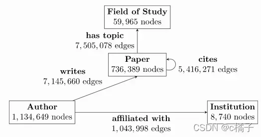
- writes(写作):作者写一篇特定的论文
- affiliated with(附属于):作者附属于某一特定机构
- cites(引用):一篇论文引用另一篇论文
- has topic(有主题):一篇论文有一个特定研究领域的主题
这个图的任务是根据图中存储的信息推断出每一篇论文(会议或期刊)的发表地点。
构建异质图
首先,我们可以创建 torch_geometric.data.HeteroData类型的数据对象,为每种类型分别定义节点特征张量、边索引张量和边特征张量:
from torch_geometric.data import HeteroData

data = HeteroData() # 实例化一个空对象

# 初始化结点特征
data['paper'].x = ... # [num_papers, num_features_paper]
data['author'].x = ... # [num_authors, num_features_author]
data['institution'].x = ... # [num_institutions, num_features_institution]
data['field_of_study'].x = ... # [num_field, num_features_field]
# 初始化边索引
data['paper', 'cites', 'paper'].edge_index = ... # [2, num_edges_cites]
data['author', 'writes', 'paper'].edge_index = ... # [2, num_edges_writes]
data['author', 'affiliated_with', 'institution'].edge_index = ... # [2, num_edges_affiliated]
data['author', 'has_topic', 'institution'].edge_index = ... # [2, num_edges_topic]
# 初始化边特征
data['paper', 'cites', 'paper'].edge_attr = ... # [num_edges_cites, num_features_cites]
data['author', 'writes', 'paper'].edge_attr = ... # [num_edges_writes, num_features_writes]
data['author', 'affiliated_with', 'institution'].edge_attr = ... # [num_edges_affiliated, num_features_affiliated]
data['paper', 'has_topic', 'field_of_study'].edge_attr = ... # [num_edges_topic, num_features_topic]
节点或边张量将在第一次访问时自动创建,并由字符串类型的键索引。节点类型由单个字符串标识,而边缘类型由字符串的三元组 (source_node_type, edge_type, destination_node_type)标识:边缘类型标识符和边缘类型可以存在的两个节点类型。并且,数据对象允许每种类型有不同的特征维度。
包含按属性名而不是按节点或边类型分组的异构信息的字典可以通过 data.{attribute_name}_dict直接访问,并作为输入到GNN模型中:
model = HeteroGNN(...)
# 下面是数据对象调用方式
output = model(data.x_dict, data.edge_index_dict, data.edge_attr_dict)
如果该数据集存在于PyG数据集列表中,则可以直接导入和使用。并且它将被下载到根目录并自动处理。
from torch_geometric.datasets import OGB_MAG

dataset = OGB_MAG(root='./data', preprocess='metapath2vec')
data = dataset[0]
数据对象可以打印出来进行验证。
HeteroData(
  paper={
    x=[736389, 128],
    y=[736389],
    train_mask=[736389],
    val_mask=[736389],
    test_mask=[736389]
  },
  author={ x=[1134649, 128] },
  institution={ x=[8740, 128] },
  field_of_study={ x=[59965, 128] },
  (author, affiliated_with, institution)={ edge_index=[2, 1043998] },
  (author, writes, paper)={ edge_index=[2, 7145660] },
  (paper, cites, paper)={ edge_index=[2, 5416271] },
  (paper, has_topic, field_of_study)={ edge_index=[2, 7505078] }
)
utility函数
torch_geometric.data.HeteroData类提供了许多有用的实用函数来修改和分析给定的图。
例如,单个节点或边存储可以被单独索引:
paper_node_data = data['paper']
cites_edge_data = data['paper', 'cites', 'paper']
我们可以添加新的节点类型或张量,并删除它们:
data['paper'].year = ...    # Setting a new paper attribute
del data['field_of_study']  # Deleting 'field_of_study' node type
del data['has_topic']       # Deleting 'has_topic' edge type
我们可以访问数据对象的元数据,包含所有当前节点和边缘类型的信息:
node_types, edge_types = data.metadata()
print(node_types)
['paper', 'author', 'institution']
print(edge_types)
[('paper', 'cites', 'paper'),
('author', 'writes', 'paper'),
('author', 'affiliated_with', 'institution')]
数据对象可以像往常一样在设备之间传输:
data = data.to('cuda:0')
data = data.cpu()
我们还可以使用其他辅助函数来分析给定的图
data.has_isolated_nodes()
data.has_self_loops()
data.is_undirected()
并且可以通过 to_homogeneous()将其转换为同构的“类型化”图,该图能够在不同类型之间保持特征的维数匹配:
homogeneous_data = data.to_homogeneous()
print(homogeneous_data)
Data(x=[1879778, 128], edge_index=[2, 13605929], edge_type=[13605929])
在这里,homogeneous_data.Edge_type表示一个边级向量,以整数形式保存每条边的边类型。
异构图 transformations
大多数用于预处理规则图的 transformations也适用于异构图数据对象。
import torch_geometric.transforms as T

data = T.ToUndirected()(data)
data = T.AddSelfLoops()(data)
data = T.NormalizeFeatures()(data)
这里,ToUndirected()通过为图中的所有边添加反向边,将有向图转换为无向图。消息传递将在所有边的两个方向上执行。
对于所有类型为 node_type的节点和所有现有形式的边缘类型 ('node_type', 'edge_type', 'node_type'),函数 AddSelfLoops()将添加自循环边。因此,在消息传递期间,每个节点可能从自身接收一个或多个消息(每个适当的边类型接收一个消息)。
NormalizeFeatures()的工作方式与同质情况类似,并将所有指定的特征归并为1。
创建异构图神经网络
标准消息传递gnn (Standard Message Passing gnn, mp – gnn)不能简单地应用于异构图数据,因为不同类型的节点和边特征由于特征类型的不同而不能被相同的函数处理。解决这个问题的一种方法是为每个边类型分别实现消息和更新函数。在运行时,MP-GNN算法需要在消息计算期间遍历边类型字典,在节点更新期间遍历节点类型字典。
为了避免不必要的运行时开销,并使创建异构mp – gnn尽可能简单,Pytorch geometry为用户提供了三种方法来创建异构图形数据模型:
- 通过使用
torch_geometrici .nn.to_hetero()或torch_geometrici .nn.to_hetero_with_bases()自动将一个同质GNN模型转换为一个异构的GNN模型 - 使用PyGs包装器为不同类型定义单独的函数。用于异构卷积的
HeteroConv - 部署现有的(或编写自己的)异构GNN算子
下面将详细介绍每个方法:
自动转换GNN模型
Pytorch geometry允许使用内置函数 torch_geometrical .nn.to_hetero()或 torch_geometrical .nn.to_hetero_with_bases()自动将任何PyG GNN模型转换为异构输入图形的模型。
import torch_geometric.transforms as T
from torch_geometric.datasets import OGB_MAG
from torch_geometric.nn import SAGEConv, to_hetero

# 读取数据集 并自动预处理为无向图
dataset = OGB_MAG(root='./data', preprocess='metapath2vec', transform=T.ToUndirected())
data = dataset[0]

class GNN(torch.nn.Module):
    def __init__(self, hidden_channels, out_channels):
        super().__init__()
        self.conv1 = SAGEConv((-1, -1), hidden_channels)
        self.conv2 = SAGEConv((-1, -1), out_channels)

    def forward(self, x, edge_index):
        x = self.conv1(x, edge_index).relu()
        x = self.conv2(x, edge_index)
        return x


model = GNN(hidden_channels=64, out_channels=dataset.num_classes)
model = to_hetero(model, data.metadata(), aggr='sum')
该过程采用一个现有的GNN模型,并复制消息函数以分别处理每个边类型,如下图所示。
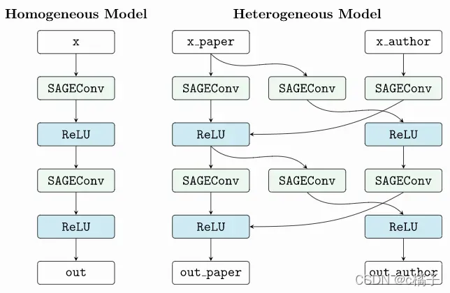
因此,该模型现在期望将节点和边类型作为键作为输入参数的字典,而不是在同构图中使用的单张量。注意,我们将in_channels的元组传递给SAGEConv,以便允许在二分图中传递消息。
由于输入特性的数量和张量的大小因不同类型而异,PyG可以利用延迟初始化来初始化异构gnn中的参数(用-1表示in_channels参数)。这允许我们避免计算和跟踪计算图的所有张量大小。所有现有的PyG操作符都支持延迟初始化。我们可以通过调用一次来初始化模型的参数:
with torch.no_grad():  # Initialize lazy modules.
    out = model(data.x_dict, data.edge_index_dict)
to_hetero()和 to_hetero_with_bases()对于可以自动转换为异构体系结构的同构体系结构来说都非常灵活。举个例子:
from torch_geometric.nn import GATConv, Linear, to_hetero
# 定义模型 全部延迟初始化
class GAT(torch.nn.Module):
    def __init__(self, hidden_channels, out_channels):
        super().__init__()
        self.conv1 = GATConv((-1, -1), hidden_channels, add_self_loops=False)
        self.lin1 = Linear(-1, hidden_channels)
        self.conv2 = GATConv((-1, -1), out_channels, add_self_loops=False)
        self.lin2 = Linear(-1, out_channels)

    def forward(self, x, edge_index):
        x = self.conv1(x, edge_index) + self.lin1(x)
        x = x.relu()
        x = self.conv2(x, edge_index) + self.lin2(x)
        return x
# 转换
model = GAT(hidden_channels=64, out_channels=dataset.num_classes)
model = to_hetero(model, data.metadata(), aggr='sum')
通常,可以使用如下方法训练(其实和torch中一样~~,需要注意的就是传入数据的字典表示):
def train():
    model.train()
    optimizer.zero_grad()
    out = model(data.x_dict, data.edge_index_dict)
    mask = data['paper'].train_mask
    loss = F.cross_entropy(out['paper'][mask], data['paper'].y[mask])
    loss.backward()
    optimizer.step()
    return float(loss)
使用异构卷积包装器
异构卷积卷积包装器 torch_geometric.nn.conv.HeteroConv允许定义自定义异构消息和更新函数,以从头开始为异构图构建任意mp – gnn。虽然 to_hetero()自动转换器对所有边类型使用相同的操作,但包装器允许为不同的边类型定义不同的操作。HeteroConv接受一个子模块字典作为输入,图数据中的每一种边类型都有一个。下面的示例演示如何应用它。
from torch_geometric.nn import HeteroConv, GCNConv, SAGEConv, GATConv, Linear

class HeteroGNN(torch.nn.Module):
    def __init__(self, hidden_channels, out_channels, num_layers):
        super().__init__()

        self.convs = torch.nn.ModuleList()
        for _ in range(num_layers):
            conv = HeteroConv({
                ('paper', 'cites', 'paper'): GCNConv(-1, hidden_channels),
                ('author', 'writes', 'paper'): SAGEConv((-1, -1), hidden_channels),
                ('paper', 'rev_writes', 'author'): GATConv((-1, -1), hidden_channels),
            }, aggr='sum')
            self.convs.append(conv)

        self.lin = Linear(hidden_channels, out_channels)

    def forward(self, x_dict, edge_index_dict):
	# 需要注意的就是这里需要传入字典
        for conv in self.convs:
            x_dict = conv(x_dict, edge_index_dict)
            x_dict = {key: x.relu() for key, x in x_dict.items()}
        return self.lin(x_dict['author'])

model = HeteroGNN(hidden_channels=64, out_channels=dataset.num_classes,
                  num_layers=2)

with torch.no_grad():  # Initialize lazy modules.
     out = model(data.x_dict, data.edge_index_dict)
部署现有的异构算子
PyG提供了操作符(例如,torch_geometrical.nn.convt.hgtconv),这是专门为异构图设计的。这些操作符可以直接用于构建异构的GNN模型,如下例所示:
from torch_geometric.nn import HGTConv, Linear

class HGT(torch.nn.Module):
    def __init__(self, hidden_channels, out_channels, num_heads, num_layers):
        super().__init__()
	# 将各种类型的边使用线性层转换为同一个维度
        self.lin_dict = torch.nn.ModuleDict()
        for node_type in data.node_types:
            self.lin_dict[node_type] = Linear(-1, hidden_channels)

	# 堆叠多层异构卷积层 num_heads是使用了多头注意力机制
        self.convs = torch.nn.ModuleList()
        for _ in range(num_layers):
            conv = HGTConv(hidden_channels, hidden_channels, data.metadata(),num_heads, group='sum')
            self.convs.append(conv)

        self.lin = Linear(hidden_channels, out_channels)

    def forward(self, x_dict, edge_index_dict):
        for node_type, x in x_dict.items():
            x_dict[node_type] = self.lin_dict[node_type](x).relu_()

        for conv in self.convs:
            x_dict = conv(x_dict, edge_index_dict)

        return self.lin(x_dict['author'])

model = HGT(hidden_channels=64, out_channels=dataset.num_classes,
            num_heads=2, num_layers=2)

with torch.no_grad():  # Initialize lazy modules.
     out = model(data.x_dict, data.edge_index_dict)
异构图采样
PyG为异构图形的采样提供了各种功能,例如在标准的 torch_geometric.loader.NeighborLoader类或专用的异构图形采样器,如 torch_geometric.loader.HGTLoader。这对于大型异构图的高效表示学习特别有用,因为在这种情况下,处理完整数量的邻居的计算开销太大。对其他采样器(如 torch_geometrical.loader.ClusterLoader,torch_geometric.loader.GraphSAINTLoader)的异构图形支持很快就会加入。总的来说,所有异构图形加载器都将生成一个 HeteroData对象作为输出,其中包含原始数据的一个子集,其主要不同之处是其采样过程的工作方式。因此,将训练过程从全批处理转换为小批处理只需要很小的代码更改。
使用 NeighborLoader进行邻居采样的工作原理如下:
import torch_geometric.transforms as T
from torch_geometric.datasets import OGB_MAG
from torch_geometric.loader import NeighborLoader

transform = T.ToUndirected()  # Add reverse edge types.
data = OGB_MAG(root='./data', preprocess='metapath2vec', transform=transform)[0]

train_loader = NeighborLoader(
    data,
    # Sample 15 neighbors for each node and each edge type for 2 iterations:
    num_neighbors=[15] * 2,
    # Use a batch size of 128 for sampling training nodes of type "paper":
    batch_size=128,
    input_nodes=('paper', data['paper'].train_mask),
)

batch = next(iter(train_loader))
NeighborLoader既适用于同构图,也适用于异构图。当在异构图中操作时,可以对单个边类型的采样邻居数量进行更细粒度的控制,但不是必需的,例如:
num_neighbors = {key: [15] * 2 for key in data.edge_types}
打印 Batch,然后产生以下输出:
HeteroData(
  paper={
    x=[20799, 256],
    y=[20799],
    train_mask=[20799],
    val_mask=[20799],
    test_mask=[20799],
    batch_size=128
  },
  author={ x=[4419, 128] },
  institution={ x=[302, 128] },
  field_of_study={ x=[2605, 128] },
  (author, affiliated_with, institution)={ edge_index=[2, 0] },
  (author, writes, paper)={ edge_index=[2, 5927] },
  (paper, cites, paper)={ edge_index=[2, 11829] },
  (paper, has_topic, field_of_study)={ edge_index=[2, 10573] },
  (institution, rev_affiliated_with, author)={ edge_index=[2, 829] },
  (paper, rev_writes, author)={ edge_index=[2, 5512] },
  (field_of_study, rev_has_topic, paper)={ edge_index=[2, 10499] }
)
batch共有28187个节点,用于计算128个“paper”节点的嵌入。被采样的节点总是根据它们被采样的顺序进行排序。因此,batch['paper'].batch_size节点表示原始的mini-batch节点集合,便于通过切片获得最终的输出嵌入。
在小批处理模式下训练我们的异构GNN模型与在全批处理模式下训练类似,只是我们通过 train_loader迭代生成的mini-batch,并基于单个mini-batch小批处优化模型参数:
def train():
    model.train()

    total_examples = total_loss = 0
    for batch in train_loader:
        optimizer.zero_grad()
        batch = batch.to('cuda:0')
        batch_size = batch['paper'].batch_size
        out = model(batch.x_dict, batch.edge_index_dict)
        loss = F.cross_entropy(out['paper'][:batch_size],
                               batch['paper'].y[:batch_size])
        loss.backward()
        optimizer.step()

        total_examples += batch_size
        total_loss += float(loss) * batch_size

    return total_loss / total_examples
重要的是,在损失计算过程中,我们只使用了前128个“paper”节点。我们基于 batch['paper'].batch_size,对labels batch['paper'.y和输出 out['paper']来表示原始mini-batch的标签和输出。
参考链接
loss.backward()
optimizer.step()
    total_examples += batch_size
    total_loss += float(loss) * batch_size

return total_loss / total_examples
重要的是,在损失计算过程中,我们只使用了前128个“paper”节点。我们基于 batch['paper'].batch_size,对labels batch['paper'.y和输出 out['paper']来表示原始mini-batch的标签和输出。
文章出处登录后可见!