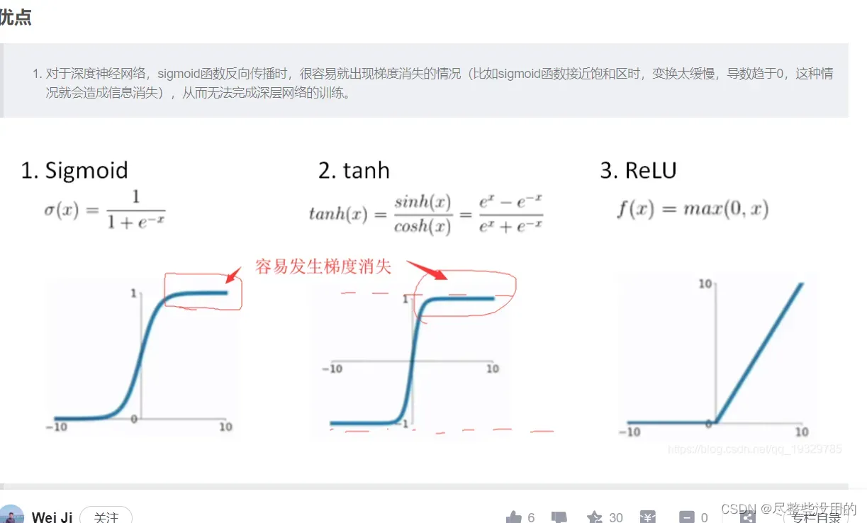
开篇先告诉自己一件事,nerf用的是最快的relu激活,因为relu没有梯度消失现象,所以快,
至于这种现象的解释请看下图(还有elu和prelu这两个梯度保留的更好,nerf跑一跑?嘻嘻!):
ok,开始谈谈mlp,mlp实际上就是一个拥有多层神经网络的所谓多层感知机,感知机都是用来分类的

由上图可知mlp最大的作用就是可以实现非线性的分类,而为什么可进行非线性分类,就是因为这个隐藏层进行了空间的转换,也就是我前一篇博客说的为了实现非线性必须要的操作。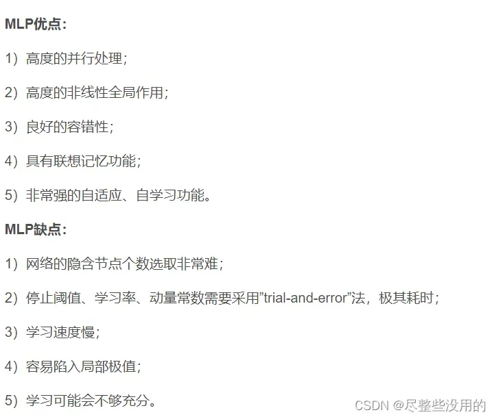
mlp缺点也挺多的,速度慢算一个,难怪nerf跑得这么慢 ,给一个转载自其他人博客的mlp代码在这:
from __future__ import print_function, division
import numpy as np
import math
from sklearn import datasets
from mlfromscratch.utils import train_test_split, to_categorical, normalize, accuracy_score, Plot
from mlfromscratch.deep_learning.activation_functions import Sigmoid, Softmax
from mlfromscratch.deep_learning.loss_functions import CrossEntropy
class MultilayerPerceptron():
“””Multilayer Perceptron classifier. A fully-connected neural network with one hidden layer.
Unrolled to display the whole forward and backward pass.
Parameters:
———–
n_hidden: int:
The number of processing nodes (neurons) in the hidden layer.
n_iterations: float
The number of training iterations the algorithm will tune the weights for.
learning_rate: float
The step length that will be used when updating the weights.
“””
def __init__(self, n_hidden, n_iterations=3000, learning_rate=0.01):
self.n_hidden = n_hidden
self.n_iterations = n_iterations
self.learning_rate = learning_rate
self.hidden_activation = Sigmoid()
self.output_activation = Softmax()
self.loss = CrossEntropy()
def _initialize_weights(self, X, y):
n_samples, n_features = X.shape
_, n_outputs = y.shape
# Hidden layer
limit = 1 / math.sqrt(n_features)
self.W = np.random.uniform(-limit, limit, (n_features, self.n_hidden))
self.w0 = np.zeros((1, self.n_hidden))
# Output layer
limit = 1 / math.sqrt(self.n_hidden)
self.V = np.random.uniform(-limit, limit, (self.n_hidden, n_outputs))
self.v0 = np.zeros((1, n_outputs))
def fit(self, X, y):
self._initialize_weights(X, y)
for i in range(self.n_iterations):
# …………..
# Forward Pass
# …………..
# HIDDEN LAYER
hidden_input = X.dot(self.W) + self.w0
hidden_output = self.hidden_activation(hidden_input)
# OUTPUT LAYER
output_layer_input = hidden_output.dot(self.V) + self.v0
y_pred = self.output_activation(output_layer_input)
# ……………
# Backward Pass
# ……………
# OUTPUT LAYER
# Grad. w.r.t input of output layer
grad_wrt_out_l_input = self.loss.gradient(y, y_pred) * self.output_activation.gradient(output_layer_input)
grad_v = hidden_output.T.dot(grad_wrt_out_l_input)
grad_v0 = np.sum(grad_wrt_out_l_input, axis=0, keepdims=True)
# HIDDEN LAYER
# Grad. w.r.t input of hidden layer
grad_wrt_hidden_l_input = grad_wrt_out_l_input.dot(self.V.T) * self.hidden_activation.gradient(hidden_input)
grad_w = X.T.dot(grad_wrt_hidden_l_input)
grad_w0 = np.sum(grad_wrt_hidden_l_input, axis=0, keepdims=True)
# Update weights (by gradient descent)
# Move against the gradient to minimize loss
self.V -= self.learning_rate * grad_v
self.v0 -= self.learning_rate * grad_v0
self.W -= self.learning_rate * grad_w
self.w0 -= self.learning_rate * grad_w0
# Use the trained model to predict labels of X
def predict(self, X):
# Forward pass:
hidden_input = X.dot(self.W) + self.w0
hidden_output = self.hidden_activation(hidden_input)
output_layer_input = hidden_output.dot(self.V) + self.v0
y_pred = self.output_activation(output_layer_input)
return y_pred
def main():
data = datasets.load_digits()
X = normalize(data.data)
y = data.target
# Convert the nominal y values to binary
y = to_categorical(y)
X_train, X_test, y_train, y_test = train_test_split(X, y, test_size=0.4, seed=1)
# MLP
clf = MultilayerPerceptron(n_hidden=16,
n_iterations=1000,
learning_rate=0.01)
clf.fit(X_train, y_train)
y_pred = np.argmax(clf.predict(X_test), axis=1)
y_test = np.argmax(y_test, axis=1)
accuracy = accuracy_score(y_test, y_pred)
print (“Accuracy:”, accuracy)
# Reduce dimension to two using PCA and plot the results
Plot().plot_in_2d(X_test, y_pred, title=”Multilayer Perceptron”, accuracy=accuracy, legend_labels=np.unique(y))
if __name__ == “__main__”:
main()
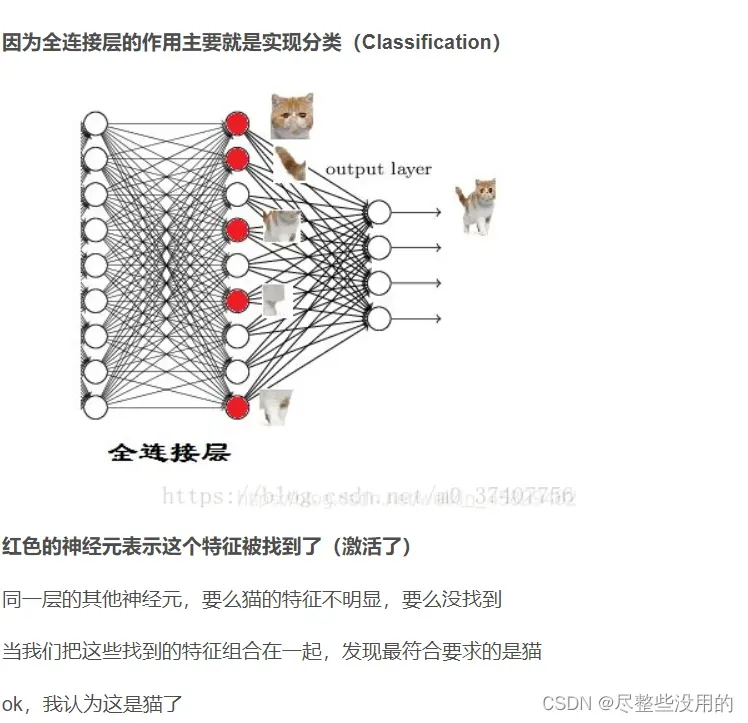
这里的隐藏层是全连接层,因为这个隐藏层要换x的空间肯定是要作用于全部的x上,在卷积网络上也有全连接层但那个和这个的意思不太一样(全连接只是表示这一层于上一层所有神经元都连接了,根据各个神经元的参数不同,全连接层的作用自然也是不同的),卷积里的是用来分类,
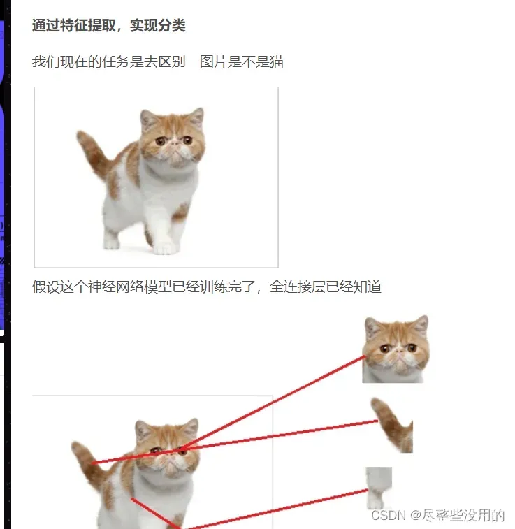
这里全连接层的神经元是激活函数(可能有点语义表达错误和sigmoid那些应该不一样,刚看了一下是一样的,因为前一层神经元要先经过全连接层处理,然后经过激活函数处理,使用就是由激活函数判断它是否激活某个条件,我看Alex net用的是relu激活(这个函数在同样数据下激活态会多一点,我觉得可能是因为非饱和,值的范围比较大导致的,不过relu在梯度下降方面表现的似乎不错,先不管这个了))。
你如果前一层的神经元和权重的组合达到了一定的条件,那么这一层的某些神经元就会被激活(达到激活函数的条件了),最后的输出层只要把这些激活的东西拼在一起看是什么就行(当然这个拼起来的结果在数学上的表示是一个抽象值,这点我在之前的博客说过,得到了这个值就可以把它和我训练出来的猫的决策分界的值进行对比,就可以知道是不是猫了)。
有人跟我说全连接的输出维度如果小于输入维度(他称这个为隐层,我觉得和隐藏层的概念不同)是为了更好的拟合,我觉得有道理,减小了输入那原来的特征就只能被迫组合,这样也就必须出来一个组合后的产物(有点像数学上的拟合过程),叫拟合是正常的。放一个转载的连接层代码,方便理解:
import torch.nn as nn
import torch.nn.functional as F
class Net(nn.Module):
def __init__(self):
#nn.Module子类的函数必须在构建函数中执行父类的构造函数
#下式等价于nn.Module.__init__(self)
super(Net, self).__init__()
#卷积层“1”表示输入图片为单通道,“6”表示输出通道数,‘5’表示卷积核为5*5
self.conv1 = nn.Conv2d(1, 6, 5)
#卷积层
self.conv2 = nn.Conv2d(6, 16, 5)
#全连接层,y=Wx+b
self.fc1 = nn.Linear(16*5*5, 120)
#参考第三节,这里第一层的核大小是前一层卷积层的输出和核大小16*5*5,一共120层
self.fc2 = nn.Linear(120, 84)
#接下来每一层的核大小为1*1
self.fc3 = nn.Linear(84, 10)
def forward(self, x):
#卷积–激活–池化
x = F.max_pool2d(F.relu(self.conv1(x)), (2, 2))
x = F.max_pool2d(F.relu(self.conv2(x)), 2)
#reshape ,’-1’表示自适应
x = x.view(x.size()[0], -1)
x = F.relu(self.fc1(x))
x = F.relu(self.fc2(x))
x = self.fc3
return x
net = Net()
print(net)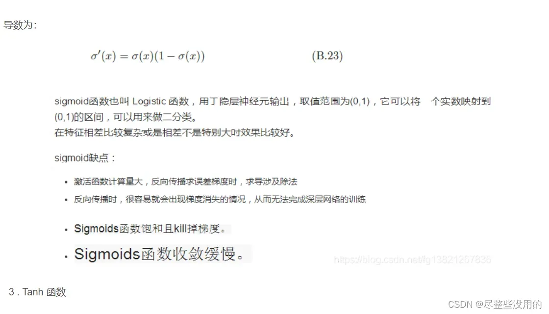
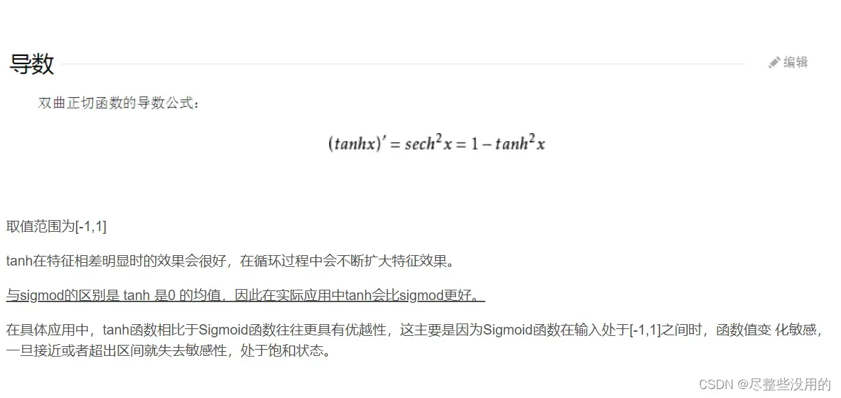

我觉得这几个函数的特点我都要放一下,方便我以后清楚他们各自的作用。
文章出处登录后可见!