文章目录

一、前言

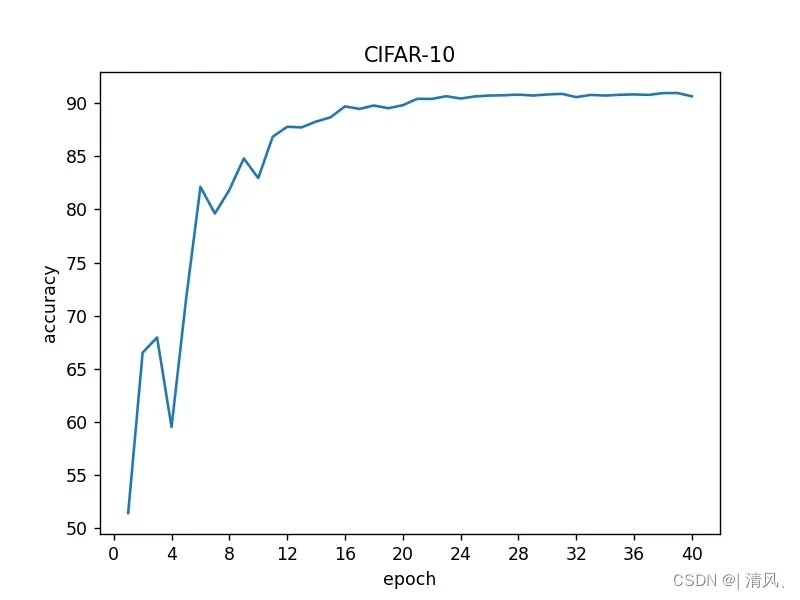
刚入门卷积神经网络，在cifar-10数据集上复现了LeNet、AlexNet和VGG-16网络，发现VGG-16网络分类准确率最高，之后以VGG-16网络为基础疯狂调参，最终达到了90.97%的准确率。（继续进行玄学调参，可以更高）

二、VGG-16网络介绍

VGGNet是牛津大学视觉几何组（Visual Geometry Group)提出的模型，原文链接：VGG-16论文该模型在2014年的ILSVRC中取得了分类任务第二、定位任务第一的优异成绩。

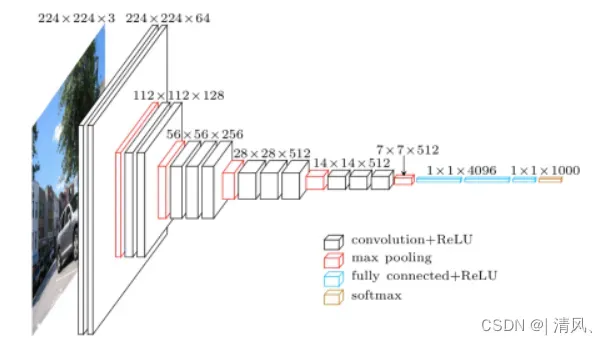
整体架构上，VGG的一大特点是在卷积层中统一使用了3×3的小卷积核和2×2大小的小池化核，层数更深，特征图更宽，证明了多个小卷积核的堆叠比单一大卷积核带来了精度提升，同时也降低了计算量。

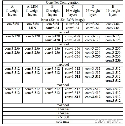
在论文中，作者给出了5种VGGNet模型，层数分别是11,11,13,16,19，最后两种卷积神经网络即是常见的VGG-16以及VGG-19.该模型的主要缺点在于参数量有140M之多，需要更大的存储空间。

三、VGG-16网络搭建与训练

3.1 网络结构搭建

搭建VGG-16网络，代码如下：

import torch
import torchvision
import torchvision.transforms as transforms
import torch.nn as nn
import torch.optim as optim
import torch.nn.functional as F
import numpy as np
import matplotlib.pyplot as plt

transform_train = transforms.Compose(
    [transforms.Pad(4),
     transforms.ToTensor(),
     transforms.Normalize((0.485, 0.456, 0.406), (0.229, 0.224, 0.225)),
     transforms.RandomHorizontalFlip(),
     transforms.RandomGrayscale(),
     transforms.RandomCrop(32, padding=4),
])

transform_test = transforms.Compose(
    [
     transforms.ToTensor(),
     transforms.Normalize((0.485, 0.456, 0.406), (0.229, 0.224, 0.225))]
)

device = torch.device("cuda:0" if torch.cuda.is_available() else "cpu")

trainset = torchvision.datasets.CIFAR10(root='dataset_method_1', train=True, download=True, transform=transform_train)
trainLoader = torch.utils.data.DataLoader(trainset, batch_size=24, shuffle=True)

testset = torchvision.datasets.CIFAR10(root='dataset_method_1', train=False, download=True, transform=transform_test)
testLoader = torch.utils.data.DataLoader(testset, batch_size=24, shuffle=False)

vgg = [96, 96, 'M', 128, 128, 'M', 256, 256, 256, 'M', 512, 512, 512, 'M', 512, 512, 512, 'M']


class VGG(nn.Module):
    def __init__(self, vgg):
        super(VGG, self).__init__()
        self.features = self._make_layers(vgg)
        self.dense = nn.Sequential(
            nn.Linear(512, 4096),
            nn.ReLU(inplace=True),
            nn.Dropout(0.4),
            nn.Linear(4096, 4096),
            nn.ReLU(inplace=True),
            nn.Dropout(0.4),
        )
        self.classifier = nn.Linear(4096, 10)

    def forward(self, x):
        out = self.features(x)
        out = out.view(out.size(0), -1)
        out = self.dense(out)
        out = self.classifier(out)
        return out

    def _make_layers(self, vgg):
        layers = []
        in_channels = 3
        for x in vgg:
            if x == 'M':
                layers += [nn.MaxPool2d(kernel_size=2, stride=2)]
            else:
                layers += [nn.Conv2d(in_channels, x, kernel_size=3, padding=1),
                           nn.BatchNorm2d(x),
                           nn.ReLU(inplace=True)]
                in_channels = x

        layers += [nn.AvgPool2d(kernel_size=1, stride=1)]
        return nn.Sequential(*layers)

该结构相比传统的VGG-16有一些小小的改动：

（1）前两层卷积神经网络中把通道数从64改为了96。（玄学调参，准确率有一丁点的提升）

（2）在全连接层中把每一层的神经元Dropout概率从0.5调成了0.4。对于Dropout的概率值，个人感觉在该数据集中设为0.5并不是一个较好的选择，这会使得最后训练过程中的running_loss卡在400-500之间，无论把学习率调得多小也学不动了。在准确率上的体现就是，Dropout设为0.5时模型在测试集上的分类准确率一直在卡在89%左右，无法突破90%，而设为0.4之后就立刻提升到了接近91%，running_loss最终降到300左右。据此推测，继续调整Dropout参数可以让该模型的准确率在此基础上进一步提升（在此并没有尝试）。

在搭建该网络的过程中总结出的一些心得体会：

（1）对图像的预处理、数据增强的工作要做好。这可以让训练集更丰富，就像在五年高考真题中又衍生出了三年模拟题让神经网络学习，可以让模型更具有泛化能力，防止过拟合。根据原数据集的特点进行合适的数据增强（并不是所有的数据增强操作都可以提升准确率，有些操作加了反而会使得准确率下降），对分类准确率的提升是立竿见影的。

（2）batch_size不要设得太小。一开始的时候batch_size的值设成了4，结果一轮epoch需要训练12000次，即使用GPU跑也很耗时间。设成了24就比之前的快得多了（当然还可以设得更大一些）

3.2 模型训练

代码如下：

model = VGG(vgg)
# model.load_state_dict(torch.load('CIFAR-model/VGG16.pth'))
optimizer = optim.SGD(model.parameters(), lr=0.01, weight_decay=5e-3)
loss_func = nn.CrossEntropyLoss()
scheduler = optim.lr_scheduler.StepLR(optimizer, step_size=5, gamma=0.4, last_epoch=-1)


total_times = 40
total = 0
accuracy_rate = []


def test():
    model.eval()
    correct = 0  # 预测正确的图片数
    total = 0  # 总共的图片数
    with torch.no_grad():
        for data in testLoader:
            images, labels = data
            images = images.to(device)
            outputs = model(images).to(device)
            outputs = outputs.cpu()
            outputarr = outputs.numpy()
            _, predicted = torch.max(outputs, 1)
            total += labels.size(0)
            correct += (predicted == labels).sum()
    accuracy = 100 * correct / total
    accuracy_rate.append(accuracy)
    print(f'准确率为:{accuracy}%'.format(accuracy))


for epoch in range(total_times):
    model.train()
    model.to(device)
    running_loss = 0.0
    total_correct = 0
    total_trainset = 0

    for i, (data, labels) in enumerate(trainLoader, 0):
        data = data.to(device)
        outputs = model(data).to(device)
        labels = labels.to(device)
        loss = loss_func(outputs, labels).to(device)
        optimizer.zero_grad()
        loss.backward()
        optimizer.step()
        running_loss += loss.item()
        _, pred = outputs.max(1)
        correct = (pred == labels).sum().item()
        total_correct += correct
        total_trainset += data.shape[0]
        running_loss += loss.item()
        if i % 1000 == 0 and i > 0:
            print(f"正在进行第{i}次训练, running_loss={running_loss}".format(i, running_loss))
            running_loss = 0.0
    test()
    scheduler.step()


# torch.save(model.state_dict(), 'CIFAR-model/VGG16.pth')
accuracy_rate = np.array(accuracy_rate)
times = np.linspace(1, total_times, total_times)
plt.xlabel('times')
plt.ylabel('accuracy rate')
plt.plot(times, accuracy_rate)
plt.show()

print(accuracy_rate)

在训练网络的过程中总结出的一些心得体会：

（1）优化器使用SGD更好些，Adam一开始收敛速度确实较快，但是后期可能会出现模型难以收敛的情况。

（2）引入scheduler对学习率进行动态调整非常有效。训练初期为了加速收敛，可以把学习率设得大一些，在此设成了0.01，running_loss下降得很快；而在训练中后期，需要使用更小的学习率来一点点地推进。为了实现这种效果，第一种方案是不断保存模型的参数，之后修手动修改学习率再加载参数继续训练，第二种方案是使用lr_scheduler提供的各种动态调整方案进行动态调整。在此使用StepLR等间隔调整学习率，总的epoch是40次，每隔5次将学习率调整为原来的0.4（玄学调参）。在训练过程中可以很明显地看到，每隔5个epoch调整学习率之后，分类准确率相比上一个epoch突然有了很大的提升。

3.3 训练结果

完整代码如下：

import torch
import torchvision
import torchvision.transforms as transforms
import torch.nn as nn
import torch.optim as optim
import torch.nn.functional as F
import numpy as np
import matplotlib.pyplot as plt

transform_train = transforms.Compose(
    [transforms.Pad(4),
     transforms.ToTensor(),
     transforms.Normalize((0.485, 0.456, 0.406), (0.229, 0.224, 0.225)),
     transforms.RandomHorizontalFlip(),
     transforms.RandomGrayscale(),
     transforms.RandomCrop(32, padding=4),
])

transform_test = transforms.Compose(
    [
     transforms.ToTensor(),
     transforms.Normalize((0.485, 0.456, 0.406), (0.229, 0.224, 0.225))]
)

device = torch.device("cuda:0" if torch.cuda.is_available() else "cpu")

trainset = torchvision.datasets.CIFAR10(root='dataset_method_1', train=True, download=True, transform=transform_train)
trainLoader = torch.utils.data.DataLoader(trainset, batch_size=24, shuffle=True)

testset = torchvision.datasets.CIFAR10(root='dataset_method_1', train=False, download=True, transform=transform_test)
testLoader = torch.utils.data.DataLoader(testset, batch_size=24, shuffle=False)

vgg = [96, 96, 'M', 128, 128, 'M', 256, 256, 256, 'M', 512, 512, 512, 'M', 512, 512, 512, 'M']


class VGG(nn.Module):
    def __init__(self, vgg):
        super(VGG, self).__init__()
        self.features = self._make_layers(vgg)
        self.dense = nn.Sequential(
            nn.Linear(512, 4096),
            nn.ReLU(inplace=True),
            nn.Dropout(0.4),
            nn.Linear(4096, 4096),
            nn.ReLU(inplace=True),
            nn.Dropout(0.4),
        )
        self.classifier = nn.Linear(4096, 10)

    def forward(self, x):
        out = self.features(x)
        out = out.view(out.size(0), -1)
        out = self.dense(out)
        out = self.classifier(out)
        return out

    def _make_layers(self, vgg):
        layers = []
        in_channels = 3
        for x in vgg:
            if x == 'M':
                layers += [nn.MaxPool2d(kernel_size=2, stride=2)]
            else:
                layers += [nn.Conv2d(in_channels, x, kernel_size=3, padding=1),
                           nn.BatchNorm2d(x),
                           nn.ReLU(inplace=True)]
                in_channels = x

        layers += [nn.AvgPool2d(kernel_size=1, stride=1)]
        return nn.Sequential(*layers)


model = VGG(vgg)
# model.load_state_dict(torch.load('CIFAR-model/VGG16.pth'))
optimizer = optim.SGD(model.parameters(), lr=0.01, weight_decay=5e-3)
loss_func = nn.CrossEntropyLoss()
scheduler = optim.lr_scheduler.StepLR(optimizer, step_size=5, gamma=0.4, last_epoch=-1)


total_times = 40
total = 0
accuracy_rate = []


def test():
    model.eval()
    correct = 0  # 预测正确的图片数
    total = 0  # 总共的图片数
    with torch.no_grad():
        for data in testLoader:
            images, labels = data
            images = images.to(device)
            outputs = model(images).to(device)
            outputs = outputs.cpu()
            outputarr = outputs.numpy()
            _, predicted = torch.max(outputs, 1)
            total += labels.size(0)
            correct += (predicted == labels).sum()
    accuracy = 100 * correct / total
    accuracy_rate.append(accuracy)
    print(f'准确率为:{accuracy}%'.format(accuracy))


for epoch in range(total_times):
    model.train()
    model.to(device)
    running_loss = 0.0
    total_correct = 0
    total_trainset = 0

    for i, (data, labels) in enumerate(trainLoader, 0):
        data = data.to(device)
        outputs = model(data).to(device)
        labels = labels.to(device)
        loss = loss_func(outputs, labels).to(device)
        optimizer.zero_grad()
        loss.backward()
        optimizer.step()
        running_loss += loss.item()
        _, pred = outputs.max(1)
        correct = (pred == labels).sum().item()
        total_correct += correct
        total_trainset += data.shape[0]
        running_loss += loss.item()
        if i % 1000 == 0 and i > 0:
            print(f"正在进行第{i}次训练, running_loss={running_loss}".format(i, running_loss))
            running_loss = 0.0
    test()
    scheduler.step()


# torch.save(model.state_dict(), 'CIFAR-model/VGG16.pth')
accuracy_rate = np.array(accuracy_rate)
times = np.linspace(1, total_times, total_times)
plt.xlabel('times')
plt.ylabel('accuracy rate')
plt.plot(times, accuracy_rate)
plt.show()

print(accuracy_rate)

下面附上运行上述代码在测试集上得到的分类准确率变化折线图：

四、总结

VGG网络确实算是古董了，如果想进一步提升准确率，可以考虑使用ResNet之类的结构。2022年发表的论文里把cifar-10分类的准确率做到了99.612%，实在是太猛了……

文章出处登录后可见！

已经登录？立即刷新

pytorch——使用VGG-16实现cifar-10多分类，准确率90.97%