Github源码:facebookresearch/detr
Github注释版源码:HuKai97/detr-annotations
论文:End-to-End Object Detection with Transformers
转载:【DETR源码解析】
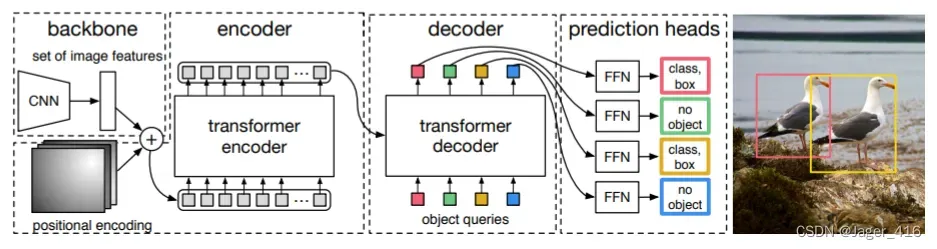
概述
DETR 即 DEtection TRansformer, 是 Facebook AI 研究院提出的 CV 模型,主要用于目标检测,也可以用于分割任务。该模型使用 Transformer 替代了复杂的目标检测传统套路,比如 two-stage 或 one-stage、anchor-based 或 anchor-free、nms 后处理等;也没有使用一些骚里骚气的技巧,比如在使用多尺度特征融合、使用一些特殊类型的卷积(如分组卷积、可变性卷积、动态生成卷积等)来抽取特征、对特征图作不同类型的映射以将分类与回归任务解耦、甚至是数据增强,整个过程就是使用CNN提取特征后编码解码得到预测输出。
可以说,整体工作很solid,虽然效果未至于 SOTA,但将炼丹者们通常认为是属于 NLP 领域的 Transformer 拿来跨界到 CV 领域使用,并且能work,这是具有重大意义的,其中的思想也值得我们学习。这种突破传统与开创时代的工作往往是深得人心的,比如 Faster R-CNN 和 YOLO,你可以看到之后的许多工作都是在它们的基础上做改进的。
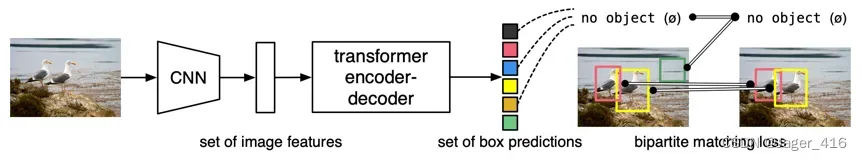
概括地说,DETR 将目标检测任务看作集合预测问题, 对于一张图片,固定预测一定数量的物体(原作是100个,在代码中可更改),模型根据这些物体对象与图片中全局上下文的关系直接并行输出预测集, 也就是 Transformer 一次性解码出图片中所有物体的预测结果,这种并行特性使得 DETR 非常高效。
特点:
- 端到端:去除了NMS和Anchor,没有那么多的超参数,计算量的大大减少,整个网络变得很简单;
- 基于Transformer:首次将Transformer引入到目标检测任务当中;
- 提出一种新的基于集合的损失函数:通过二分图匹配的方法强制模型输出一组独一无二的预测框,每个物体只会产生一个预测框,这样就讲目标检测问题之间转换为集合预测问题,所以才不用NMS,达到端到端的效果;
- 而且在decoder输入一组科学的object query和encoder输出的全局上线特征,直接以并行方式强制最终输出的100个预测框,替代了anchor;
缺点: - 对大物体的检测效果很好,但是对小物体的监测效果不是很好;训练起来比较慢;
- 由于query的设计以及初始化等问题,DETR模型从零开始训练需要超长的训练时间;
优点: - 在COCO数据集上速度和精度和Faster RCNN差不多;可以扩展到很多细分的任务中,比如分割、追踪、多模态等;
流程:
- 输入图像进过CNN网络后得到图像的特征矩阵;
- 将图像拉直并添加位置编码;
- 输入Transformer encoder中学习特征的相关性信息;
- 将encoder输出以及object query作为decoder的输入得到解码后的信息;
- 将解码后的信息传入FFN得到预测信息;
- 判断FFN预测信息是否包含真实的目标对象;
- 如果有,则输出预测框和类别,否则输出一个no object类。
原理
基于集合预测的损失函数
二分图匹配确定有效预测框
预测得到N(100)个预测框,gt为M个框,通常N>M,那么怎么计算损失呢?
这里呢,就先对这100个预测框和gt框进行一个二分图的匹配,先确定每个gt对应的是哪个预测框,最终再计算M个预测框和M个gt框的总损失。
其实很简单,假设现在有一个矩阵,横坐标就是我们预测的100个预测框,纵坐标就是gt框,分别计算每个预测框和其他所有gt框的cost,这样就构成了一个cost matrix,再确定把如何把所有gt框分配给对应的预测框,才能使得最终的总cost最小。
这里计算的方法就是很经典的匈牙利算法,通常是调用scipy包中的linear_sum_assignment函数来完成。这个函数的输入就是cost matrix,输出一组行索引和一个对应的列索引,给出最佳分配。
所以通过以上的步骤,就确定了最终100个预测框中哪些预测框会作为有效预测框,哪些预测框会称为背景。再将有效预测框和gt框计算最终损失(有效预测框个数等于gt框个数)。
损失函数
损失函数:分类损失+回归损失
分类损失:交叉熵损失,去掉log
回归损失:GIOU Loss + L1 Loss
源码
整体结构
-
Backbone:
- 作用:提取图像特征,并将图像尺度缩小
- 结构:Resnet
- 输入:一个batch的image [B, 3, W, H]
- 输出:Resnet50最后一层的feature map [B, 2048, W_feat, H_feat]
-
过渡层:
- 作用:将backbone的输出转换为encoder所需要的shape,同时准备Transformer所需的其他变量,如masks、positional_embedding等
-
Transformer:
- 结构:encoder、decoder
- 总输入:
- x:输入的feature map [B, 256, W_feat, H_feat]
- mask:encoder和decoder中的有效padding mask [B, W_feat, H_feat]
- query_embed:decoder中的query的嵌入向量 [num_query(100), 256]
- positional_embedding:iamge feature的位置编码嵌入向量,encoder中的query_pos,decoder中的key_pos [B, 256, W_feat, H_feat]
- 总输出:
- out_dec:decoder的输出**(目标query输出)****[num_dec_layers(6), B, num_query(100), 256]**,虽然我们将decoder所有层的输出都保留了下来,但是我们想要的最终的输出只有decoder layer的最后一层输出
- memory:encoder的输出 [B, 256, W_feat, H_feat]
-
Transformer中的Encoder:
- 作用:对feature map进行位置编码和self attention,通过自注意力聚合feature map全局的特征
- 结构:self_attention、normalization、feed forward network、normalization
- 输入:
- query:输入query,是展平后的feature map [W_feat*H_feat, B, 256]
- value、key:在self attention中,k和v是由q算出,因此输入为None
- query_key_padding_mask:feature map的有效padding mask [B, W_feat*H_feat]
- query_positional_embedding:feature map的位置编码 [W_feat*H_feat, B, 256]
- 输出:
- encoder_out:输出经过自注意力的展平feature map [W_feat*H_feat, B, 256]
-
Transformer中的Decoder:
- 作用:
- 第一部分是对object query进行self attention,使得每个object query关注不同的obejct信息
- 第二部分是将object query与encoder_out进行cross attention,让object query在feature map上找到不同的obejct
- 结构:
- self attention(self_attention、normalization)
- cross attention(cross_attention、normalization、feed forward network、normalization)
- self attention:
- 输入:
- query:初始化object query [num_layer(6), num_query(100), B, 256]
- key、value:在self attention中,k和v是由q计算得到,None
- query_positional_embedding: query的位置编码 [num_layer(6), num_query(100), B, 256]
- mask:在decoder的self attention中,没有mask的输入 None
- 输出:
- 经过自注意力的object query [num_layer(6), num_query(100), B, 256]
- 输入:
- cross attention:
- 输入:
- query:经过自注意力得到的object query,即self attention模块的输出 [num_layer(6), num_query(100), B, 256]
- key、value:cross attention中,k和v都是encoder的输出 [N, B, 256]
- query_positional_embedding: query的位置编码 [num_layer(6), num_query(100), B, 256]
- key_positional_embedding:key的位置编码,即feature map的位置编码 [W_feat*H_feat**, **B, 256]
- key_padding_mask: key,即feature map的有效padding mask [B, W_feat*H_feat]
- 输出:
- out_dec:decoder的输出 [num_layers(6), B, num_query(100), 256]
- memory:encoder的输出 [W_feat*H_feat, B, 256]
- 输入:
- 作用:
模型搭建过程分为:
- 搭建DETR:Backbone + Transformer + MLP(Multilayer Perceptron,多层神经网络)
- 初始化损失函数:criterion + 初始化后处理:postprocessors
def build(args):
    # the `num_classes` naming here is somewhat misleading.
    # it indeed corresponds to `max_obj_id + 1`, where max_obj_id
    # is the maximum id for a class in your dataset. For example,
    # COCO has a max_obj_id of 90, so we pass `num_classes` to be 91.
    # As another example, for a dataset that has a single class with id 1,
    # you should pass `num_classes` to be 2 (max_obj_id + 1).
    # For more details on this, check the following discussion
    # https://github.com/facebookresearch/detr/issues/108#issuecomment-650269223
    # 最大类别ID+1
    num_classes = 20 if args.dataset_file != 'coco' else 91
    if args.dataset_file == "coco_panoptic":
        # for panoptic, we just add a num_classes that is large enough to hold
        # max_obj_id + 1, but the exact value doesn't really matter
        num_classes = 250
    device = torch.device(args.device)

    # 搭建backbone resnet + PositionEmbeddingSine
    backbone = build_backbone(args)

    # 搭建transformer
    transformer = build_transformer(args)

    # 搭建整个DETR模型
    model = DETR(
        backbone,
        transformer,
        num_classes=num_classes,
        num_queries=args.num_queries,
        aux_loss=args.aux_loss,
    )

    # 是否需要额外的分割任务
    if args.masks:
        model = DETRsegm(model, freeze_detr=(args.frozen_weights is not None))

    # HungarianMatcher()  二分图匹配
    matcher = build_matcher(args)

    # 损失权重
    weight_dict = {'loss_ce': 1, 'loss_bbox': args.bbox_loss_coef}
    weight_dict['loss_giou'] = args.giou_loss_coef
    if args.masks:   # 分割任务  False
        weight_dict["loss_mask"] = args.mask_loss_coef
        weight_dict["loss_dice"] = args.dice_loss_coef
    # TODO this is a hack
    if args.aux_loss:   # 辅助损失  每个decoder都参与计算损失  True
        aux_weight_dict = {}
        for i in range(args.dec_layers - 1):
            aux_weight_dict.update({k + f'_{i}': v for k, v in weight_dict.items()})
        weight_dict.update(aux_weight_dict)

    losses = ['labels', 'boxes', 'cardinality']
    if args.masks:
        losses += ["masks"]

    # 定义损失函数
    criterion = SetCriterion(num_classes, matcher=matcher, weight_dict=weight_dict,
                             eos_coef=args.eos_coef, losses=losses)
    criterion.to(device)

    # 定义后处理
    postprocessors = {'bbox': PostProcess()}

    # 分割
    if args.masks:
        postprocessors['segm'] = PostProcessSegm()
        if args.dataset_file == "coco_panoptic":
            is_thing_map = {i: i <= 90 for i in range(201)}
            postprocessors["panoptic"] = PostProcessPanoptic(is_thing_map, threshold=0.85)

    return model, criterion, postprocessors
搭建模型
class DETR(nn.Module):
    """ This is the DETR module that performs object detection """
    def __init__(self, backbone, transformer, num_classes, num_queries, aux_loss=False):
        """ Initializes the model.
        Parameters:
            backbone: torch module of the backbone to be used. See backbone.py
            transformer: torch module of the transformer architecture. See transformer.py
            num_classes: number of object classes
            num_queries: number of object queries, ie detection slot. This is the maximal number of objects
                         DETR can detect in a single image. For COCO, we recommend 100 queries.
            aux_loss: True if auxiliary decoding losses (loss at each decoder layer) are to be used.
        """
        super().__init__()
        self.num_queries = num_queries
        self.transformer = transformer
        hidden_dim = transformer.d_model
        # 分类
        self.class_embed = nn.Linear(hidden_dim, num_classes + 1)
        # 回归
        self.bbox_embed = MLP(hidden_dim, hidden_dim, 4, 3)
        # self.query_embed 类似于传统目标检测里面的anchor 这里设置了100个  [100,256]
        # nn.Embedding 等价于 nn.Parameter
        self.query_embed = nn.Embedding(num_queries, hidden_dim)
        self.input_proj = nn.Conv2d(backbone.num_channels, hidden_dim, kernel_size=1)
        self.backbone = backbone
        self.aux_loss = aux_loss   # True

    def forward(self, samples: NestedTensor):
        """ The forward expects a NestedTensor, which consists of:
               - samples.tensor: batched images, of shape [batch_size x 3 x H x W]
               - samples.mask: a binary mask of shape [batch_size x H x W], containing 1 on padded pixels

            It returns a dict with the following elements:
               - "pred_logits": the classification logits (including no-object) for all queries.
                                Shape= [batch_size x num_queries x (num_classes + 1)]
               - "pred_boxes": The normalized boxes coordinates for all queries, represented as
                               (center_x, center_y, height, width). These values are normalized in [0, 1],
                               relative to the size of each individual image (disregarding possible padding).
                               See PostProcess for information on how to retrieve the unnormalized bounding box.
               - "aux_outputs": Optional, only returned when auxilary losses are activated. It is a list of
                                dictionnaries containing the two above keys for each decoder layer.
        """
        if isinstance(samples, (list, torch.Tensor)):
            samples = nested_tensor_from_tensor_list(samples)
        # out: list{0: tensor=[bs,2048,19,26] + mask=[bs,19,26]}  经过backbone resnet50 block5输出的结果
        # pos: list{0: [bs,256,19,26]}  位置编码
        features, pos = self.backbone(samples)

        # src: Tensor [bs,2048,19,26]
        # mask: Tensor [bs,19,26]
        src, mask = features[-1].decompose()
        assert mask is not None

        # 数据输入transformer进行前向传播
        # self.input_proj(src) [bs,2048,19,26]->[bs,256,19,26]
        # mask: False的区域是不需要进行注意力计算的
        # self.query_embed.weight  类似于传统目标检测里面的anchor 这里设置了100个
        # pos[-1]  位置编码  [bs, 256, 19, 26]
        # hs: [6, bs, 100, 256]
        hs = self.transformer(self.input_proj(src), mask, self.query_embed.weight, pos[-1])[0]

        # 分类 [6个decoder, bs, 100, 256] -> [6, bs, 100, 92(类别)]
        outputs_class = self.class_embed(hs)
        # 回归 [6个decoder, bs, 100, 256] -> [6, bs, 100, 4]
        outputs_coord = self.bbox_embed(hs).sigmoid()
        out = {'pred_logits': outputs_class[-1], 'pred_boxes': outputs_coord[-1]}
        if self.aux_loss:   # True
            out['aux_outputs'] = self._set_aux_loss(outputs_class, outputs_coord)
        # dict: 3
        # 0 pred_logits 分类头输出[bs, 100, 92(类别数)]
        # 1 pred_boxes 回归头输出[bs, 100, 4]
        # 3 aux_outputs list: 5  前5个decoder层输出 5个pred_logits[bs, 100, 92(类别数)] 和 5个pred_boxes[bs, 100, 4]
        return out

    @torch.jit.unused
    def _set_aux_loss(self, outputs_class, outputs_coord):
        # this is a workaround to make torchscript happy, as torchscript
        # doesn't support dictionary with non-homogeneous values, such
        # as a dict having both a Tensor and a list.
        return [{'pred_logits': a, 'pred_boxes': b}
                for a, b in zip(outputs_class[:-1], outputs_coord[:-1])]
Backbone
Backbone主要包括CNN特征提取和位置编码两个部分。
首先是调用models/Backbone.py中的build_backbone函数创建Backbone:
def build_backbone(args):
    # 搭建backbone
    # 位置编码  PositionEmbeddingSine()
    position_embedding = build_position_encoding(args)
    train_backbone = args.lr_backbone > 0   # 是否需要训练backbone  True
    return_interm_layers = args.masks       # 是否需要返回中间层结果 目标检测False  分割True
    # 生成backbone  resnet50
    backbone = Backbone(args.backbone, train_backbone, return_interm_layers, args.dilation)
    # 将backbone输出与位置编码相加   0: backbone   1: PositionEmbeddingSine()
    model = Joiner(backbone, position_embedding)
    model.num_channels = backbone.num_channels   # 512
    return model
这里首先调用build_position_encoding函数生成正余弦位置编码position_embedding:[batchsize,256,H/32, W/32],其中256前128是y方向位置编码,后128是x方向位置编码;再调用Backbone类生成ResNet50对输入数据进行特征提取得到特征图[batchsize,2048,H/32, W/32]。最后Joiner将两者合并存储起来,方便后续使用。
CNN
创建ResNet50,先调用Backbone类:
class Backbone(BackboneBase):
    """ResNet backbone with frozen BatchNorm."""
    def __init__(self, name: str,
                 train_backbone: bool,
                 return_interm_layers: bool,
                 dilation: bool):
        # 直接掉包 调用torchvision.models中的backbone
        backbone = getattr(torchvision.models, name)(
            replace_stride_with_dilation=[False, False, dilation],
            pretrained=is_main_process(), norm_layer=FrozenBatchNorm2d)
        # resnet50  2048
        num_channels = 512 if name in ('resnet18', 'resnet34') else 2048
        super().__init__(backbone, train_backbone, num_channels, return_interm_layers)
这个类是继承自BackboneBase类的,而且CNN直接调用的就是torchvision.models中的模型,所以直接看BackboneBase类
class BackboneBase(nn.Module):

    def __init__(self, backbone: nn.Module, train_backbone: bool, num_channels: int, return_interm_layers: bool):
        super().__init__()
        for name, parameter in backbone.named_parameters():
            # layer0 layer1不需要训练 因为前面层提取的信息其实很有限 都是差不多的 不需要训练
            if not train_backbone or 'layer2' not in name and 'layer3' not in name and 'layer4' not in name:
                parameter.requires_grad_(False)
        # False 检测任务不需要返回中间层
        if return_interm_layers:
            return_layers = {"layer1": "0", "layer2": "1", "layer3": "2", "layer4": "3"}
        else:
            return_layers = {'layer4': "0"}
        # 检测任务直接返回layer4即可  执行torchvision.models._utils.IntermediateLayerGetter这个函数可以直接返回对应层的输出结果
        self.body = IntermediateLayerGetter(backbone, return_layers=return_layers)
        self.num_channels = num_channels

    def forward(self, tensor_list: NestedTensor):
        """
        tensor_list: pad预处理之后的图像信息
        tensor_list.tensors: [bs, 3, 608, 810]预处理后的图片数据 对于小图片而言多余部分用0填充
        tensor_list.mask: [bs, 608, 810] 用于记录矩阵中哪些地方是填充的(原图部分值为False,填充部分值为True)
        """
        # 取出预处理后的图片数据 [bs, 3, 608, 810] 输入模型中  输出layer4的输出结果 dict '0'=[bs, 2048, 19, 26]
        xs = self.body(tensor_list.tensors)
        # 保存输出数据
        out: Dict[str, NestedTensor] = {}
        for name, x in xs.items():
            m = tensor_list.mask  # 取出图片的mask [bs, 608, 810] 知道图片哪些区域是有效的 哪些位置是pad之后的无效的
            assert m is not None
            # 通过插值函数知道卷积后的特征的mask  知道卷积后的特征哪些是有效的  哪些是无效的
            # 因为之前图片输入网络是整个图片都卷积计算的 生成的新特征其中有很多区域都是无效的
            mask = F.interpolate(m[None].float(), size=x.shape[-2:]).to(torch.bool)[0]
            # out['0'] = NestedTensor: tensors[bs, 2048, 19, 26] + mask[bs, 19, 26]
            out[name] = NestedTensor(x, mask)
        # out['0'] = NestedTensor: tensors[bs, 2048, 19, 26] + mask[bs, 19, 26]
        return out
这个类还是在调用torchvision.models中的模型,然后再把预处理后的图片数据[bs, 3, 608, 810]和mask数据[bs, 608, 810]输入到模型中(这个图片数据是经过pad填充的数据,而mask数据就是记录这些图片哪些像素位置是pad的,为True,没用pad的真实有效数据就为False)。经过前向传播,再调用IntermediateLayerGetter函数把对应层特征图提取出来,得到原图32倍下采样的特征图[bs, 2048, 19, 26],以及这张特征图对应的mask[bs, 19, 26]。
Positional Encoding
Positional Encoding 就是位置编码。这里主要是调用models/position_encoding.py中的build_position_encoding函数创建位置编码:
def build_position_encoding(args):
    """
    创建位置编码
    args: 一系列参数  args.hidden_dim: transformer中隐藏层的维度   args.position_embedding: 位置编码类型 正余弦sine or 可学习learned
    """
    # N_steps = 128 = 256 // 2  backbone输出[bs,256,25,34]  256维度的特征
    # 而传统的位置编码应该也是256维度的, 但是detr用的是一个x方向和y方向的位置编码concat的位置编码方式  这里和ViT有所不同
    # 二维位置编码   前128维代表x方向位置编码  后128维代表y方向位置编码
    N_steps = args.hidden_dim // 2
    if args.position_embedding in ('v2', 'sine'):
        # TODO find a better way of exposing other arguments
        # [bs,256,19,26]  dim=1时  前128个是y方向位置编码  后128个是x方向位置编码
        position_embedding = PositionEmbeddingSine(N_steps, normalize=True)
    elif args.position_embedding in ('v3', 'learned'):
        position_embedding = PositionEmbeddingLearned(N_steps)
    else:
        raise ValueError(f"not supported {args.position_embedding}")

    return position_embedding
可以看到,源码是实现了两种位置编码,一种是正余弦绝对位置编码,不需要额外的参数学习,另一种是可学习绝对位置编码。原论文用的是正余弦绝对位置编码,而且代码也是默认使用这个的,所以这里主要介绍PositionEmbeddingSine类:
class PositionEmbeddingSine(nn.Module):
    """
    Absolute pos embedding, Sine.  没用可学习参数  不可学习  定义好了就固定了
    This is a more standard version of the position embedding, very similar to the one
    used by the Attention is all you need paper, generalized to work on images.
    """
    def __init__(self, num_pos_feats=64, temperature=10000, normalize=False, scale=None):
        super().__init__()
        self.num_pos_feats = num_pos_feats    # 128维度  x/y  = d_model/2
        self.temperature = temperature        # 常数 正余弦位置编码公式里面的10000
        self.normalize = normalize            # 是否对向量进行max规范化   True
        if scale is not None and normalize is False:
            raise ValueError("normalize should be True if scale is passed")
        if scale is None:
            # 这里之所以规范化到2*pi  因为位置编码函数的周期是[2pi, 20000pi]
            scale = 2 * math.pi  # 规范化参数 2*pi
        self.scale = scale

    def forward(self, tensor_list: NestedTensor):
        x = tensor_list.tensors   # [bs, 2048, 19, 26]  预处理后的 经过backbone 32倍下采样之后的数据  对于小图片而言多余部分用0填充
        mask = tensor_list.mask   # [bs, 19, 26]  用于记录矩阵中哪些地方是填充的(原图部分值为False,填充部分值为True)
        assert mask is not None
        not_mask = ~mask   # True的位置才是真实有效的位置

        # 考虑到图像本身是2维的 所以这里使用的是2维的正余弦位置编码
        # 这样各行/列都映射到不同的值 当然有效位置是正常值 无效位置会有重复值 但是后续计算注意力权重会忽略这部分的
        # 而且最后一个数字就是有效位置的总和,方便max规范化
        # 计算此时y方向上的坐标  [bs, 19, 26]
        y_embed = not_mask.cumsum(1, dtype=torch.float32)
        # 计算此时x方向的坐标    [bs, 19, 26]
        x_embed = not_mask.cumsum(2, dtype=torch.float32)

        # 最大值规范化 除以最大值 再乘以2*pi 最终把坐标规范化到0-2pi之间
        if self.normalize:
            eps = 1e-6
            y_embed = y_embed / (y_embed[:, -1:, :] + eps) * self.scale
            x_embed = x_embed / (x_embed[:, :, -1:] + eps) * self.scale

        dim_t = torch.arange(self.num_pos_feats, dtype=torch.float32, device=x.device)   # 0 1 2 .. 127
        # 2i/2i+1: 2 * (dim_t // 2)  self.temperature=10000   self.num_pos_feats = d/2
        dim_t = self.temperature ** (2 * (dim_t // 2) / self.num_pos_feats)   # 分母

        pos_x = x_embed[:, :, :, None] / dim_t   # 正余弦括号里面的公式
        pos_y = y_embed[:, :, :, None] / dim_t   # 正余弦括号里面的公式
        # x方向位置编码: [bs,19,26,64][bs,19,26,64] -> [bs,19,26,64,2] -> [bs,19,26,128]
        pos_x = torch.stack((pos_x[:, :, :, 0::2].sin(), pos_x[:, :, :, 1::2].cos()), dim=4).flatten(3)
        # y方向位置编码: [bs,19,26,64][bs,19,26,64] -> [bs,19,26,64,2] -> [bs,19,26,128]
        pos_y = torch.stack((pos_y[:, :, :, 0::2].sin(), pos_y[:, :, :, 1::2].cos()), dim=4).flatten(3)
        # concat: [bs,19,26,128][bs,19,26,128] -> [bs,19,26,256] -> [bs,256,19,26]
        pos = torch.cat((pos_y, pos_x), dim=3).permute(0, 3, 1, 2)

        # [bs,256,19,26]  dim=1时  前128个是y方向位置编码  后128个是x方向位置编码
        return pos
对照公式:
我的几个关键点的理解:
- 这里是通过mask来构建位置编码的,mask中记录了特征图中每个像素位置是否是pad的,只有在为False的位置,才是有效的位置,才需要构建位置编码;
- 关于最大值规范化 :因为正余弦编码方式,思想就是将各个位置的通过公式映射到 0~2Π 这个范围内(也可以是4Π,6Π,8Π…,因为它是一个周期函数,不过我们一般默认为2Π),所以这里在带入公式之前需要对x_embed、y_embed先进行规范化;
- 关于位置编码方式:这里之所以是把x和y分别进行位置编码(二维位置编码),而不是像transformer那样的一维位置编码。主要考虑的是transformer是应用在语言模型中的,天然就是一维的,所以一维可能更适合,而DETR是应用在图像任务中的一个目标检测框架,在图像任务中,当然二维位置编码效果可能会更好点;
- 这样,对于每个位置(x,y),其所在列对应的编码值就在通道维度的前128维,其所在行的编码值就在通道这个维度的后128维。这样这个特征图上各个位置就都对应到不同的维度的编码值了。
当然作为学习,也可以看看第二种绝对位置编码方式:可学习位置编码:
class PositionEmbeddingLearned(nn.Module):
    """
    Absolute pos embedding, learned.
    可以发现整个类其实就是初始化了相应shape的位置编码参数,让后通过可学习的方式学习这些位置编码参数
    """
    def __init__(self, num_pos_feats=256):
        super().__init__()
        # nn.Embedding  相当于 nn.Parameter  其实就是初始化函数
        self.row_embed = nn.Embedding(50, num_pos_feats)
        self.col_embed = nn.Embedding(50, num_pos_feats)
        self.reset_parameters()

    def reset_parameters(self):
        nn.init.uniform_(self.row_embed.weight)
        nn.init.uniform_(self.col_embed.weight)

    def forward(self, tensor_list: NestedTensor):
        x = tensor_list.tensors
        h, w = x.shape[-2:]   # 特征图h w
        i = torch.arange(w, device=x.device)
        j = torch.arange(h, device=x.device)
        x_emb = self.col_embed(i)   # 初始化x方向位置编码
        y_emb = self.row_embed(j)   # 初始化y方向位置编码
        # concat x y 方向位置编码
        pos = torch.cat([
            x_emb.unsqueeze(0).repeat(h, 1, 1),
            y_emb.unsqueeze(1).repeat(1, w, 1),
        ], dim=-1).permute(2, 0, 1).unsqueeze(0).repeat(x.shape[0], 1, 1, 1)
        return pos
可以发现整个类其实就是初始化了相应shape的位置编码参数,然后通过可学习的方式自己学习这些位置编码参数,代码比较简单。
Transformer
整体结构
先看下调用接口:
def build_transformer(args):
    return Transformer(
        d_model=args.hidden_dim,
        dropout=args.dropout,
        nhead=args.nheads,
        dim_feedforward=args.dim_feedforward,
        num_encoder_layers=args.enc_layers,
        num_decoder_layers=args.dec_layers,
        normalize_before=args.pre_norm,
        return_intermediate_dec=True,
    )
直接调用Transformer类:
class Transformer(nn.Module):

    def __init__(self, d_model=512, nhead=8, num_encoder_layers=6,
                 num_decoder_layers=6, dim_feedforward=2048, dropout=0.1,
                 activation="relu", normalize_before=False,
                 return_intermediate_dec=False):
        super().__init__()
        """
        d_model: 编码器里面mlp(前馈神经网络  2个linear层)的hidden dim 512
        nhead: 多头注意力头数 8
        num_encoder_layers: encoder的层数 6
        num_decoder_layers: decoder的层数 6
        dim_feedforward: 前馈神经网络的维度 2048
        dropout: 0.1
        activation: 激活函数类型 relu
        normalize_before: 是否使用前置LN
        return_intermediate_dec: 是否返回decoder中间层结果  False
        """
        # 初始化一个小encoder
        encoder_layer = TransformerEncoderLayer(d_model, nhead, dim_feedforward,
                                                dropout, activation, normalize_before)
        encoder_norm = nn.LayerNorm(d_model) if normalize_before else None
        # 创建整个Encoder层  6个encoder层堆叠
        self.encoder = TransformerEncoder(encoder_layer, num_encoder_layers, encoder_norm)

        # 初始化一个小decoder
        decoder_layer = TransformerDecoderLayer(d_model, nhead, dim_feedforward,
                                                dropout, activation, normalize_before)
        decoder_norm = nn.LayerNorm(d_model)
        # 创建整个Decoder层  6个decoder层堆叠
        self.decoder = TransformerDecoder(decoder_layer, num_decoder_layers, decoder_norm,
                                          return_intermediate=return_intermediate_dec)

        # 参数初始化
        self._reset_parameters()

        self.d_model = d_model  # 编码器里面mlp的hidden dim 512
        self.nhead = nhead      # 多头注意力头数 8

    def _reset_parameters(self):
        for p in self.parameters():
            if p.dim() > 1:
                nn.init.xavier_uniform_(p)

    def forward(self, src, mask, query_embed, pos_embed):
        """
        src: [bs,256,19,26] 图片输入backbone+1x1conv之后的特征图
        mask: [bs, 19, 26]  用于记录特征图中哪些地方是填充的(原图部分值为False,填充部分值为True)
        query_embed: [100, 256]  类似于传统目标检测里面的anchor  这里设置了100个   需要预测的目标
        pos_embed: [bs, 256, 19, 26]  位置编码
        """
        # bs  c=256  h=19  w=26
        bs, c, h, w = src.shape
        # src: [bs,256,19,26]=[bs,C,H,W] -> [494,bs,256]=[HW,bs,C]
        src = src.flatten(2).permute(2, 0, 1)
        # pos_embed: [bs, 256, 19, 26]=[bs,C,H,W] -> [494,bs,256]=[HW,bs,C]
        pos_embed = pos_embed.flatten(2).permute(2, 0, 1)
        # query_embed: [100, 256]=[num,C] -> [100,bs,256]=[num,bs,256]
        query_embed = query_embed.unsqueeze(1).repeat(1, bs, 1)
        # mask: [bs, 19, 26]=[bs,H,W] -> [bs,494]=[bs,HW]
        mask = mask.flatten(1)

        # tgt: [100, bs, 256] 需要预测的目标query embedding 和 query_embed形状相同  且全设置为0
        #                     在每层decoder层中不断的被refine,相当于一次次的被coarse-to-fine的过程
        tgt = torch.zeros_like(query_embed)
        # memory: [494, bs, 256]=[HW, bs, 256]  Encoder输出  具有全局相关性(增强后)的特征表示
        memory = self.encoder(src, src_key_padding_mask=mask, pos=pos_embed)
        # [6, 100, bs, 256]
        # tgt:需要预测的目标 query embeding
        # memory: encoder的输出
        # pos: memory的位置编码
        # query_pos: tgt的位置编码
        hs = self.decoder(tgt, memory, memory_key_padding_mask=mask,
                          pos=pos_embed, query_pos=query_embed)
        # decoder输出 [6, 100, bs, 256] -> [6, bs, 100, 256]
        # encoder输出 [bs, 256, H, W]
        return hs.transpose(1, 2), memory.permute(1, 2, 0).view(bs, c, h, w)
仔细分析这个类会发现,我们虽然暂时不了解模型的细节部分,但是模型的主体框架已经定义出来了。整个Transformer其实就是输入经过Backbone输出的特征图src(降维到256)、src_key_padding_mask(记录特征图每个位置是否是被pad的,pad的就不需要计算注意力)和位置编码pos到TransformerEncoder中,而TransformerEncoder其实是由TransformerEncoderLayer组成的;然后再输入encoder的输出、mask、位置编码和query编码到TransformerEncoder中,而TransformerEncoder是由TransformerDecoderLayer组成的。
所以,下面分为TransformerEncoder和TransformerDecoder两个模块来了解Transformer具体细节组成。
TransformerEncoder
这个部分就是调用_get_clones函数,复制6份TransformerEncoderLayer类,然后前向传播依次输入这6个TransformerEncoderLayer类,不断的计算特征图的自注意力,并不断的增强特征图,最终得到最强的(信息最多的)特征图output:[h*w, bs, 256]。值得注意的是,整个TransformerEncoder过程特征图的shape是不变的。
class TransformerEncoder(nn.Module):

    def __init__(self, encoder_layer, num_layers, norm=None):
        super().__init__()
        # 复制num_layers=6份encoder_layer=TransformerEncoderLayer
        self.layers = _get_clones(encoder_layer, num_layers)
        # 6层TransformerEncoderLayer
        self.num_layers = num_layers
        self.norm = norm  # layer norm

    def forward(self, src,
                mask: Optional[Tensor] = None,
                src_key_padding_mask: Optional[Tensor] = None,
                pos: Optional[Tensor] = None):
        """
        src: [h*w, bs, 256]  经过Backbone输出的特征图(降维到256)
        mask: None
        src_key_padding_mask: [h*w, bs]  记录每个特征图的每个位置是否是被pad的(True无效   False有效)
        pos: [h*w, bs, 256] 每个特征图的位置编码
        """
        output = src

        # 遍历这6层TransformerEncoderLayer
        for layer in self.layers:
            output = layer(output, src_mask=mask,
                           src_key_padding_mask=src_key_padding_mask, pos=pos)

        if self.norm is not None:
            output = self.norm(output)

        # 得到最终ENCODER的输出 [h*w, bs, 256]
        return output

def _get_clones(module, N):
    return nn.ModuleList([copy.deepcopy(module) for i in range(N)])
TransformerEncoderLayer
encoder结构图:
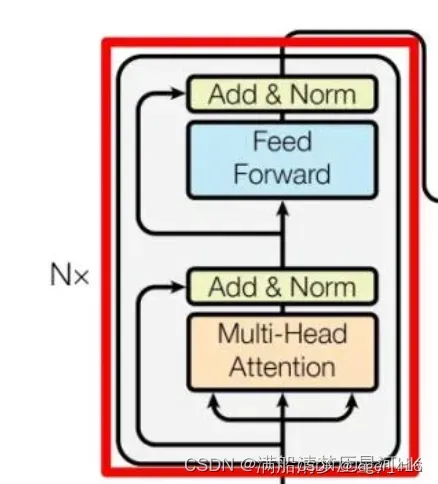
Encoder Layer = multi-head Attention + add&Norm + feed forward + add&Norm,重点在于multi-head Attention。
class TransformerEncoderLayer(nn.Module):

    def __init__(self, d_model, nhead, dim_feedforward=2048, dropout=0.1,
                 activation="relu", normalize_before=False):
        super().__init__()
        """
        小encoder层  结构:multi-head Attention + add&Norm + feed forward + add&Norm
        d_model: mlp 前馈神经网络的dim
        nhead: 8头注意力机制
        dim_feedforward: 前馈神经网络的维度 2048
        dropout: 0.1
        activation: 激活函数类型
        normalize_before: 是否使用先LN  False
        """
        self.self_attn = nn.MultiheadAttention(d_model, nhead, dropout=dropout)
        # Implementation of Feedforward model
        self.linear1 = nn.Linear(d_model, dim_feedforward)
        self.dropout = nn.Dropout(dropout)
        self.linear2 = nn.Linear(dim_feedforward, d_model)

        self.norm1 = nn.LayerNorm(d_model)
        self.norm2 = nn.LayerNorm(d_model)
        self.dropout1 = nn.Dropout(dropout)
        self.dropout2 = nn.Dropout(dropout)

        self.activation = _get_activation_fn(activation)
        self.normalize_before = normalize_before

    def with_pos_embed(self, tensor, pos: Optional[Tensor]):
        # 这个操作是把词向量和位置编码相加操作
        return tensor if pos is None else tensor + pos

    def forward_post(self,
                     src,
                     src_mask: Optional[Tensor] = None,
                     src_key_padding_mask: Optional[Tensor] = None,
                     pos: Optional[Tensor] = None):
        """
        src: [494, bs, 256]  backbone输入下采样32倍后 再 压缩维度到256的特征图
        src_mask: None
        src_key_padding_mask: [bs, 494]  记录哪些位置有pad True 没意义 不需要计算attention
        pos: [494, bs, 256]  位置编码
        """
        # 数据 + 位置编码  [494, bs, 256]
        # 这也是和原版encoder不同的地方,这里每个encoder的q和k都会加上位置编码  再用q和k计算相似度  再和v加权得到更具有全局相关性(增强后)的特征表示
        # 每用一层都加上位置编码  信息不断加强  最终得到的特征全局相关性最强  原版的transformer只在输入加上位置编码  作者发现这样更好
        q = k = self.with_pos_embed(src, pos)
        # multi-head attention   [494, bs, 256]
        # q 和 k = backbone输出特征图 + 位置编码
        # v = backbone输出特征图
        # 这里对query和key增加位置编码 是因为需要在图像特征中各个位置之间计算相似度/相关性 而value作为原图像的特征 和 相关性矩阵加权,
        # 从而得到各个位置结合了全局相关性(增强后)的特征表示,所以q 和 k这种计算需要+位置编码  而v代表原图像不需要加位置编码
        # nn.MultiheadAttention: 返回两个值  第一个是自注意力层的输出  第二个是自注意力权重  这里取0
        # key_padding_mask: 记录backbone生成的特征图中哪些是原始图像pad的部分 这部分是没有意义的
        #                   计算注意力会被填充为-inf,这样最终生成注意力经过softmax时输出就趋向于0,相当于忽略不计
        # attn_mask: 是在Transformer中用来“防作弊”的,即遮住当前预测位置之后的位置,忽略这些位置,不计算与其相关的注意力权重
        #            而在encoder中通常为None 不适用  decoder中才使用
        src2 = self.self_attn(q, k, value=src, attn_mask=src_mask,
                              key_padding_mask=src_key_padding_mask)[0]
        # add + norm + feed forward + add + norm
        src = src + self.dropout1(src2)
        src = self.norm1(src)
        src2 = self.linear2(self.dropout(self.activation(self.linear1(src))))
        src = src + self.dropout2(src2)
        src = self.norm2(src)
        return src

    def forward_pre(self, src,
                    src_mask: Optional[Tensor] = None,
                    src_key_padding_mask: Optional[Tensor] = None,
                    pos: Optional[Tensor] = None):
        src2 = self.norm1(src)
        q = k = self.with_pos_embed(src2, pos)
        src2 = self.self_attn(q, k, value=src2, attn_mask=src_mask,
                              key_padding_mask=src_key_padding_mask)[0]
        src = src + self.dropout1(src2)
        src2 = self.norm2(src)
        src2 = self.linear2(self.dropout(self.activation(self.linear1(src2))))
        src = src + self.dropout2(src2)
        return src

    def forward(self, src,
                src_mask: Optional[Tensor] = None,
                src_key_padding_mask: Optional[Tensor] = None,
                pos: Optional[Tensor] = None):
        if self.normalize_before:  # False
            return self.forward_pre(src, src_mask, src_key_padding_mask, pos)
        return self.forward_post(src, src_mask, src_key_padding_mask, pos)  # 默认执行
有几个很关键的点(和原始transformer encoder不同的地方):
- 为什么每个encoder的q和k都是+位置编码的?如果学过transformer的知道,通常都是在transformer的输入加上位置编码,而每个encoder的qkv都是相等的,都是不加位置编码的。而这里先将q和k都会加上位置编码,再用q和k计算相似度,最后和v加权得到更具有全局相关性(增强后)的特征表示。每一层都加上位置编码,每一层全局信息不断加强,最终可以得到最强的全局特征;
- 为什么q和k+位置编码,而v不需要加上位置编码?因为q和k是用来计算图像特征中各个位置之间计算相似度/相关性的,加上位置编码后计算出来的全局特征相关性更强,而v代表原图像,所以并不需要加位置编码;
TransformerDecoder
Decoder结构和Encoder的结构类似,也是用_get_clones复制6份TransformerDecoderLayer类,然后前向传播依次输入这6个TransformerDecoderLayer类,不过不同的,Decoder需要输入这6个TransformerDecoderLayer的输出,后面这6个层的输出会一起参与损失计算。
class TransformerDecoder(nn.Module):

    def __init__(self, decoder_layer, num_layers, norm=None, return_intermediate=False):
        super().__init__()
        # 复制num_layers=decoder_layer=TransformerDecoderLayer
        self.layers = _get_clones(decoder_layer, num_layers)
        self.num_layers = num_layers   # 6
        self.norm = norm               # LN
        # 是否返回中间层 默认True  因为DETR默认6个Decoder都会返回结果,一起加入损失计算的
        # 每一层Decoder都是逐层解析,逐层加强的,所以前面层的解析效果对后面层的解析是有意义的,所以作者把前面5层的输出也加入损失计算
        self.return_intermediate = return_intermediate

    def forward(self, tgt, memory,
                tgt_mask: Optional[Tensor] = None,
                memory_mask: Optional[Tensor] = None,
                tgt_key_padding_mask: Optional[Tensor] = None,
                memory_key_padding_mask: Optional[Tensor] = None,
                pos: Optional[Tensor] = None,
                query_pos: Optional[Tensor] = None):
        """
        tgt: [100, bs, 256] 需要预测的目标query embedding 和 query_embed形状相同  且全设置为0
                            在每层decoder层中不断的被refine,相当于一次次的被coarse-to-fine的过程
        memory: [h*w, bs, 256]  Encoder输出  具有全局相关性(增强后)的特征表示
        tgt_mask: None
        tgt_key_padding_mask: None
        memory_key_padding_mask: [bs, h*w]  记录Encoder输出特征图的每个位置是否是被pad的(True无效   False有效)
        pos: [h*w, bs, 256]                 特征图的位置编码
        query_pos: [100, bs, 256]    query embedding的位置编码  随机初始化的
        """
        output = tgt   # 初始化query embedding  全是0

        intermediate = []  # 用于存放6层decoder的输出结果

        # 遍历6层decoder
        for layer in self.layers:
            output = layer(output, memory, tgt_mask=tgt_mask,
                           memory_mask=memory_mask,
                           tgt_key_padding_mask=tgt_key_padding_mask,
                           memory_key_padding_mask=memory_key_padding_mask,
                           pos=pos, query_pos=query_pos)
            # 6层结果全部加入intermediate
            if self.return_intermediate:
                intermediate.append(self.norm(output))

        if self.norm is not None:
            output = self.norm(output)
            if self.return_intermediate:
                intermediate.pop()
                intermediate.append(output)
        # 默认执行这里
        # 最后把  6x[100,bs,256] -> [6(6层decoder输出),100,bs,256]
        if self.return_intermediate:
            return torch.stack(intermediate)

        return output.unsqueeze(0)   # 不执行
TransformerDecoderLayer
decoder layer 结构图:
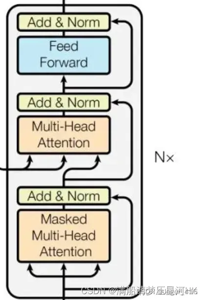
decoder layer = Masked Multi-Head Attention + Add&Norm + Multi-Head Attention + add&Norm + feed forward + add&Norm。关键点在于两个Attention层,搞懂这两层的原理、区别是理解Decoder的关键。
class TransformerDecoderLayer(nn.Module):

    def __init__(self, d_model, nhead, dim_feedforward=2048, dropout=0.1,
                 activation="relu", normalize_before=False):
        super().__init__()
        self.self_attn = nn.MultiheadAttention(d_model, nhead, dropout=dropout)
        self.multihead_attn = nn.MultiheadAttention(d_model, nhead, dropout=dropout)
        # Implementation of Feedforward model
        self.linear1 = nn.Linear(d_model, dim_feedforward)
        self.dropout = nn.Dropout(dropout)
        self.linear2 = nn.Linear(dim_feedforward, d_model)

        self.norm1 = nn.LayerNorm(d_model)
        self.norm2 = nn.LayerNorm(d_model)
        self.norm3 = nn.LayerNorm(d_model)
        self.dropout1 = nn.Dropout(dropout)
        self.dropout2 = nn.Dropout(dropout)
        self.dropout3 = nn.Dropout(dropout)

        self.activation = _get_activation_fn(activation)
        self.normalize_before = normalize_before

    def with_pos_embed(self, tensor, pos: Optional[Tensor]):
        return tensor if pos is None else tensor + pos

    def forward_post(self, tgt, memory,
                     tgt_mask: Optional[Tensor] = None,
                     memory_mask: Optional[Tensor] = None,
                     tgt_key_padding_mask: Optional[Tensor] = None,
                     memory_key_padding_mask: Optional[Tensor] = None,
                     pos: Optional[Tensor] = None,
                     query_pos: Optional[Tensor] = None):
        """
        tgt: 需要预测的目标 query embedding  负责预测物体  用于建模图像当中的物体信息  在每层decoder层中不断的被refine
             [100, bs, 256]  和 query_embed形状相同  且全设置为0
        memory: [h*w, bs, 256]  Encoder输出  具有全局相关性(增强后)的特征表示
        tgt_mask: None
        memory_mask: None
        tgt_key_padding_mask: None
        memory_key_padding_mask: [bs, h*w]  记录Encoder输出特征图的每个位置是否是被pad的(True无效   False有效)
        pos: [h*w, bs, 256]  encoder输出特征图的位置编码
        query_pos: [100, bs, 256]  query embedding/tgt的位置编码  负责建模物体与物体之间的位置关系  随机初始化的
        tgt_mask、memory_mask、tgt_key_padding_mask是防止作弊的 这里都没有使用
        """
        # 第一个self-attention的目的:找到图像中物体的信息 -> tgt
        # 第一个多头自注意力层:输入qkv都和Encoder无关  都来自于tgt/query embedding
        # 通过第一个self-attention  可以不断建模物体与物体之间的关系  可以知道图像当中哪些位置会存在物体  物体信息->tgt
        # query embedding  +  query_pos
        q = k = self.with_pos_embed(tgt, query_pos)
        # masked multi-head self-attention  计算query embedding的自注意力
        tgt2 = self.self_attn(q, k, value=tgt, attn_mask=tgt_mask,
                              key_padding_mask=tgt_key_padding_mask)[0]

        # add + norm
        tgt = tgt + self.dropout1(tgt2)
        tgt = self.norm1(tgt)

        # 第二个self-attention的目的:不断增强encoder的输出特征,将物体的信息不断加入encoder的输出特征中去,更好地表征了图像中的各个物体
        # 第二个多头注意力层,也叫Encoder-Decoder self attention:key和value来自Encoder层输出   Query来自Decoder层输入
        # 第二个self-attention 可以建模图像 与 物体之间的关系
        # 根据上一步得到的tgt作为query 不断的去encoder输出的特征图中去问(q和k计算相似度)  问图像当中的物体在哪里呢?
        # 问完之后再将物体的位置信息融合encoder输出的特征图中(和v做运算)  这样我得到的v的特征就有 encoder增强后特征信息 + 物体的位置信息
        # query = query embedding  +  query_pos
        # key = encoder输出特征 + 特征位置编码
        # value = encoder输出特征
        tgt2 = self.multihead_attn(query=self.with_pos_embed(tgt, query_pos),
                                   key=self.with_pos_embed(memory, pos),
                                   value=memory, attn_mask=memory_mask,
                                   key_padding_mask=memory_key_padding_mask)[0]
        # ada + norm + Feed Forward + add + norm
        tgt = tgt + self.dropout2(tgt2)
        tgt = self.norm2(tgt)
        tgt2 = self.linear2(self.dropout(self.activation(self.linear1(tgt))))
        tgt = tgt + self.dropout3(tgt2)
        tgt = self.norm3(tgt)

        # [100, bs, 256]
        # decoder的输出是第一个self-attention输出特征 + 第二个self-attention输出特征
        # 最终的特征:知道图像中物体与物体之间的关系 + encoder增强后的图像特征 + 图像与物体之间的关系
        return tgt

    def forward_pre(self, tgt, memory,
                    tgt_mask: Optional[Tensor] = None,
                    memory_mask: Optional[Tensor] = None,
                    tgt_key_padding_mask: Optional[Tensor] = None,
                    memory_key_padding_mask: Optional[Tensor] = None,
                    pos: Optional[Tensor] = None,
                    query_pos: Optional[Tensor] = None):
        tgt2 = self.norm1(tgt)
        q = k = self.with_pos_embed(tgt2, query_pos)
        tgt2 = self.self_attn(q, k, value=tgt2, attn_mask=tgt_mask,
                              key_padding_mask=tgt_key_padding_mask)[0]
        tgt = tgt + self.dropout1(tgt2)
        tgt2 = self.norm2(tgt)
        tgt2 = self.multihead_attn(query=self.with_pos_embed(tgt2, query_pos),
                                   key=self.with_pos_embed(memory, pos),
                                   value=memory, attn_mask=memory_mask,
                                   key_padding_mask=memory_key_padding_mask)[0]
        tgt = tgt + self.dropout2(tgt2)
        tgt2 = self.norm3(tgt)
        tgt2 = self.linear2(self.dropout(self.activation(self.linear1(tgt2))))
        tgt = tgt + self.dropout3(tgt2)
        return tgt

    def forward(self, tgt, memory,
                tgt_mask: Optional[Tensor] = None,
                memory_mask: Optional[Tensor] = None,
                tgt_key_padding_mask: Optional[Tensor] = None,
                memory_key_padding_mask: Optional[Tensor] = None,
                pos: Optional[Tensor] = None,
                query_pos: Optional[Tensor] = None):
        if self.normalize_before:
            return self.forward_pre(tgt, memory, tgt_mask, memory_mask,
                                    tgt_key_padding_mask, memory_key_padding_mask, pos, query_pos)
        return self.forward_post(tgt, memory, tgt_mask, memory_mask,
                                 tgt_key_padding_mask, memory_key_padding_mask, pos, query_pos)
总结下decoder在干嘛:
- 从Encoder的最终输出,我们得到了增强版的图像特征memory,以及特征的位置信息pos;
- 自定义了图像当中的物体信息tgt,初始化为全0,以及图像中的物体位置信息query_pos,随机初始化;
- 第一个self-attention:qk=tgt+query_pos,v=tgt,计算图像中物体与物体的相关性,负责建模图像中的物体信息,最终得到的tgt1,是增强版的物体信息,这些位置信息包含了物体与物体之间的位置关系;
- 第二个self-attention:q=tgt+qyery_pos,k=memory+pos,v=memory,以物体的信息tgt作为query,去图像特征memory中去问(计算他们的相关性),问图像中物体在哪里呢?问完之后再将物体的位置信息融入到图像特征中去(v),整个过程是负责建模图像特征与物体特征之间的关系,最后得到的是更强的图像特征tgt2,包括encoder输出的增强版的图像特征+物体的位置特征。
- 最后把tgt1 + tgt2 = Encoder输出的增强版图像特征 + 物体信息 + 物体位置信息,作为decoder的输出;
疑问一
有的人可能疑问,为什么这里定义的物体信息tgt,初始化为全0,物体位置信息query_pos,随机初始化,但是可以表示这么复杂的含义呢?它明明是初始化为全0或随机初始化的,模型怎么知道的它们代表的含义?这其实就和损失函数有关了,损失函数定义好了,通过计算损失,梯度回传,网络不断的学习,最终学习得到的tgt和query_pos就是这里表示的含义。这就和回归损失一样的,定义好了这四个channel代表xywh,那网络怎么知道的?就是通过损失函数梯度回传,网络不断学习,最终知道这四个channel就是代表xywh。
疑问二
为什么这里要将tgt1 + tgt2做为decoder的输出呢?不是单独的用tgt1或者tgt2呢?
- 首先tgt1代表图像中的物体信息 + 物体的位置信息,但是他没有太多的图像特征,这是不行的,最后预测效果肯定不好(预测物体类别肯定不是很准);
- 其次tgt2代表的encoder增强版的图像特征 + 物体的位置信息,它缺少了物体的信息,这也是不行的,最后的预测效果肯定也不好(预测物体位置肯定不是很准);
所以两者相加的特征作为decoder的输出,去预测物体的类别和位置,效果最好。
损失函数 + 后处理
损失计算:SetCriterion
首先在detr.py中会先定义好损失函数:
criterion = SetCriterion(num_classes, matcher=matcher, weight_dict=weight_dict,eos_coef=args.eos_coef, losses=losses)
criterion.to(device)
然后在engine.py的train_one_epoch中前向推理结束后调用criterion函数,计算损失:
# 前向传播
outputs = model(samples)
# 计算损失  loss_dict: 'loss_ce' + 'loss_bbox' + 'loss_giou'    用于log日志: 'class_error' + 'cardinality_error'
loss_dict = criterion(outputs, targets)
# 权重系数 {'loss_ce': 1, 'loss_bbox': 5, 'loss_giou': 2}
weight_dict = criterion.weight_dict
# 总损失 = 回归损失:loss_bbox(L1)+loss_bbox  +   分类损失:loss_ce
losses = sum(loss_dict[k] * weight_dict[k] for k in loss_dict.keys() if k in weight_dict)
好了下面着重介绍下SetCriterion类:
class SetCriterion(nn.Module):
    """ This class computes the loss for DETR.
    The process happens in two steps:
        1) we compute hungarian assignment between ground truth boxes and the outputs of the model
        2) we supervise each pair of matched ground-truth / prediction (supervise class and box)
    """
    def __init__(self, num_classes, matcher, weight_dict, eos_coef, losses):
        """ Create the criterion.
        Parameters:
            num_classes: number of object categories, omitting the special no-object category
            matcher: module able to compute a matching between targets and proposals
            weight_dict: dict containing as key the names of the losses and as values their relative weight.
            eos_coef: relative classification weight applied to the no-object category
            losses: list of all the losses to be applied. See get_loss for list of available losses.
        """
        super().__init__()
        self.num_classes = num_classes     # 数据集类别数
        self.matcher = matcher             # HungarianMatcher()  匈牙利算法 二分图匹配
        self.weight_dict = weight_dict     # dict: 18  3x6  6个decoder的损失权重   6*(loss_ce+loss_giou+loss_bbox)
        self.eos_coef = eos_coef           # 0.1
        self.losses = losses               # list: 3  ['labels', 'boxes', 'cardinality']
        empty_weight = torch.ones(self.num_classes + 1)
        empty_weight[-1] = self.eos_coef   # tensro: 92   前91=1  92=eos_coef=0.1
        self.register_buffer('empty_weight', empty_weight)

    def forward(self, outputs, targets):
        """ This performs the loss computation.
        Parameters:
             outputs: dict of tensors, see the output specification of the model for the format
                      dict: 'pred_logits'=Tensor[bs, 100, 92个class]  'pred_boxes'=Tensor[bs, 100, 4]  最后一个decoder层输出
                             'aux_output'={list:5}  0-4  每个都是dict:2 pred_logits+pred_boxes 表示5个decoder前面层的输出
             targets: list of dicts, such that len(targets) == batch_size.   list: bs
                      每张图片包含以下信息:'boxes'、'labels'、'image_id'、'area'、'iscrowd'、'orig_size'、'size'
                      The expected keys in each dict depends on the losses applied, see each loss' doc
        """
        # dict: 2   最后一个decoder层输出  pred_logits[bs, 100, 92个class] + pred_boxes[bs, 100, 4]
        outputs_without_aux = {k: v for k, v in outputs.items() if k != 'aux_outputs'}

        # 匈牙利算法  解决二分图匹配问题  从100个预测框中找到和N个gt框一一对应的预测框  其他的100-N个都变为背景
        # Retrieve the matching between the outputs of the last layer and the targets  list:1
        # tuple: 2    0=Tensor3=Tensor[5, 35, 63]  匹配到的3个预测框  其他的97个预测框都是背景
        #             1=Tensor3=Tensor[1, 0, 2]    对应的三个gt框
        indices = self.matcher(outputs_without_aux, targets)

        # Compute the average number of target boxes accross all nodes, for normalization purposes
        num_boxes = sum(len(t["labels"]) for t in targets)   # int 统计这整个batch的所有图片的gt总个数  3
        num_boxes = torch.as_tensor([num_boxes], dtype=torch.float, device=next(iter(outputs.values())).device)
        if is_dist_avail_and_initialized():
            torch.distributed.all_reduce(num_boxes)
        num_boxes = torch.clamp(num_boxes / get_world_size(), min=1).item()   # 3.0

        # 计算最后层decoder损失  Compute all the requested losses
        losses = {}
        for loss in self.losses:
            losses.update(self.get_loss(loss, outputs, targets, indices, num_boxes))

        # 计算前面5层decoder损失  累加到一起  得到最终的losses
        # In case of auxiliary losses, we repeat this process with the output of each intermediate layer.
        if 'aux_outputs' in outputs:
            for i, aux_outputs in enumerate(outputs['aux_outputs']):
                indices = self.matcher(aux_outputs, targets)   # 同样匈牙利算法匹配
                for loss in self.losses:   # 计算各个loss
                    if loss == 'masks':
                        # Intermediate masks losses are too costly to compute, we ignore them.
                        continue
                    kwargs = {}
                    if loss == 'labels':
                        # Logging is enabled only for the last layer
                        kwargs = {'log': False}
                    l_dict = self.get_loss(loss, aux_outputs, targets, indices, num_boxes, **kwargs)
                    l_dict = {k + f'_{i}': v for k, v in l_dict.items()}
                    losses.update(l_dict)
        # 参加权重更新的损失:losses: 'loss_ce' + 'loss_bbox' + 'loss_giou'    用于log日志: 'class_error' + 'cardinality_error'
        return losses
整个函数主要在做两件事:
- 调用self.matcher函数,从100个预测框中匹配出N个(gt个数)真正的预测框,匹配出每个gt框对应的预测框;
- 调用self.get_loss,计算各个损失
匈牙利算法,二分图匹配:self.matcher
匈牙利算法原理可以看看这篇经典博客:算法学习笔记(5):匈牙利算法
而在DETR是在models/matcher.py中的HungarianMatcher类实现了匈牙利匹配算法:
class HungarianMatcher(nn.Module):
    """This class computes an assignment between the targets and the predictions of the network

    For efficiency reasons, the targets don't include the no_object. Because of this, in general,
    there are more predictions than targets. In this case, we do a 1-to-1 matching of the best predictions,
    while the others are un-matched (and thus treated as non-objects).
    """

    def __init__(self, cost_class: float = 1, cost_bbox: float = 1, cost_giou: float = 1):
        """Creates the matcher

        Params:
            cost_class: This is the relative weight of the classification error in the matching cost
            cost_bbox: This is the relative weight of the L1 error of the bounding box coordinates in the matching cost
            cost_giou: This is the relative weight of the giou loss of the bounding box in the matching cost
        """
        super().__init__()
        self.cost_class = cost_class
        self.cost_bbox = cost_bbox
        self.cost_giou = cost_giou
        assert cost_class != 0 or cost_bbox != 0 or cost_giou != 0, "all costs cant be 0"

    # 不需要更新梯度  只是一种匹配方式
    @torch.no_grad()
    def forward(self, outputs, targets):
        """ Performs the matching

        Params:
            outputs: This is a dict that contains at least these entries:
                 "pred_logits": Tensor of dim [batch_size, num_queries, num_classes]=[bs,100,92] with the classification logits
                 "pred_boxes": Tensor of dim [batch_size, num_queries, 4]=[bs,100,4] with the predicted box coordinates

            targets: list:bs This is a list of targets (len(targets) = batch_size), where each target is a dict containing:
                 "labels": Tensor of dim [num_target_boxes]=[3] (where num_target_boxes is the number of ground-truth
                           objects in the target) containing the class labels
                 "boxes": Tensor of dim [num_target_boxes, 4] containing the target box coordinates

        Returns:
            A list of size batch_size, containing tuples of (index_i, index_j) where:
                - index_i is the indices of the selected predictions (in order)
                - index_j is the indices of the corresponding selected targets (in order)
            For each batch element, it holds:
                len(index_i) = len(index_j) = min(num_queries, num_target_boxes)
        """
        # batch_size  100
        bs, num_queries = outputs["pred_logits"].shape[:2]

        # We flatten to compute the cost matrices in a batch
        # [2,100,92] -> [200, 92] -> [200, 92]概率
        out_prob = outputs["pred_logits"].flatten(0, 1).softmax(-1)  # [batch_size * num_queries, num_classes]
        # [2,100,4] -> [200, 4]
        out_bbox = outputs["pred_boxes"].flatten(0, 1)  # [batch_size * num_queries, 4]

        # Also concat the target labels and boxes
        # [3]  idx = 32, 1, 85  concat all labels
        tgt_ids = torch.cat([v["labels"] for v in targets])
        # [3, 4]  concat all box
        tgt_bbox = torch.cat([v["boxes"] for v in targets])

        # 计算损失   分类 + L1 box + GIOU box
        # Compute the classification cost. Contrary to the loss, we don't use the NLL,
        # but approximate it in 1 - proba[target class].
        # The 1 is a constant that doesn't change the matching, it can be ommitted.
        cost_class = -out_prob[:, tgt_ids]

        # Compute the L1 cost between boxes
        cost_bbox = torch.cdist(out_bbox, tgt_bbox, p=1)

        # Compute the giou cost betwen boxes
        cost_giou = -generalized_box_iou(box_cxcywh_to_xyxy(out_bbox), box_cxcywh_to_xyxy(tgt_bbox))

        # Final cost matrix   [100, 3]  bs*100个预测框分别和3个gt框的损失矩阵
        C = self.cost_bbox * cost_bbox + self.cost_class * cost_class + self.cost_giou * cost_giou
        C = C.view(bs, num_queries, -1).cpu()  # [bs, 100, 3]

        sizes = [len(v["boxes"]) for v in targets]   # gt个数 3

        # 匈牙利算法进行二分图匹配  从100个预测框中挑选出最终的3个预测框 分别和gt计算损失  这个组合的总损失是最小的
        # 0: [3]  5, 35, 63   匹配到的gt个预测框idx
        # 1: [3]  1, 0, 2     对应的gt idx
        indices = [linear_sum_assignment(c[i]) for i, c in enumerate(C.split(sizes, -1))]

        # list: bs  返回bs张图片的匹配结果
        # 每张图片都是一个tuple:2
        # 0 = Tensor[gt_num,]  匹配到的正样本idx       1 = Tensor[gt_num,]  gt的idx
        return [(torch.as_tensor(i, dtype=torch.int64), torch.as_tensor(j, dtype=torch.int64)) for i, j in indices]
其实就是先计算每个预测框(100个)和每个gt框的总损失,形成损失矩阵C,然后调用scipy.optimize.linear_sum_assignment写好的匈牙利算法,匹配的原则就是 ”loss总和“ 最小(这里的loss并不是真正的loss,这里只是一种度量方式,和loss的计算方式是不一样的),得到每个gt对应的唯一负责的预测框,其他的预测框会自动归为背景。
linear_sum_assignment,输入一个二分图的度量矩阵(cost 矩阵),计算这个二分图的度量矩阵的最小权重分配方式,返回的是匹配方案对应的矩阵行索引(预测框idx)和列索引(gt框idx)。
计算损失:self.get_loss
self.get_loss是SetCriterion类定义的一个函数:
    def get_loss(self, loss, outputs, targets, indices, num_boxes, **kwargs):
        loss_map = {
            'labels': self.loss_labels,
            'cardinality': self.loss_cardinality,
            'boxes': self.loss_boxes,
            'masks': self.loss_masks
        }
        assert loss in loss_map, f'do you really want to compute {loss} loss?'
        return loss_map[loss](outputs, targets, indices, num_boxes, **kwargs)
同时会调用分类损失(self.loss_labels)、回归损失(self.boxes)和cardinality损失。不过cardinality损失只用于log,并不参与梯度更新,所以这里不展开叙述。另外如果是分割任务,这里还有一个mask分割损失计算,这里也暂时不展开叙述。
分类损失:self.loss_labels
分类损失self.loss_labels:
    def loss_labels(self, outputs, targets, indices, num_boxes, log=True):
        """Classification loss (NLL)
        targets dicts must contain the key "labels" containing a tensor of dim [nb_target_boxes]
        outputs:'pred_logits'=[bs, 100, 92] 'pred_boxes'=[bs, 100, 4] 'aux_outputs'=5*([bs, 100, 92]+[bs, 100, 4])
        targets:'boxes'=[3,4] labels=[3] ...
        indices: [3] 如:5,35,63  匹配好的3个预测框idx
        num_boxes:当前batch的所有gt个数
        """
        assert 'pred_logits' in outputs
        src_logits = outputs['pred_logits']  # 分类:[bs, 100, 92类别]

        # idx tuple:2  0=[num_all_gt] 记录每个gt属于哪张图片  1=[num_all_gt] 记录每个匹配到的预测框的index
        idx = self._get_src_permutation_idx(indices)
        target_classes_o = torch.cat([t["labels"][J] for t, (_, J) in zip(targets, indices)])
        target_classes = torch.full(src_logits.shape[:2], self.num_classes,
                                    dtype=torch.int64, device=src_logits.device)
        # 正样本+负样本  上面匹配到的预测框作为正样本 正常的idx  而100个中没有匹配到的预测框作为负样本(idx=91 背景类)
        target_classes[idx] = target_classes_o

        # 分类损失 = 正样本 + 负样本
        loss_ce = F.cross_entropy(src_logits.transpose(1, 2), target_classes, self.empty_weight)
        losses = {'loss_ce': loss_ce}

        # 日志 记录Top-1精度
        if log:
            # TODO this should probably be a separate loss, not hacked in this one here
            losses['class_error'] = 100 - accuracy(src_logits[idx], target_classes_o)[0]

        # losses: 'loss_ce': 分类损失
        #         'class_error':Top-1精度 即预测概率最大的那个类别与对应被分配的GT类别是否一致  这部分仅用于日志显示 并不参与模型训练
        return losses

    def _get_src_permutation_idx(self, indices):
        # permute predictions following indices
        # [num_all_gt]  记录每个gt都是来自哪张图片的 idx
        batch_idx = torch.cat([torch.full_like(src, i) for i, (src, _) in enumerate(indices)])
        # 记录匹配到的预测框的idx
        src_idx = torch.cat([src for (src, _) in indices])
        return batch_idx, src_idx
注意:
- 分类损失 = 交叉熵损失;
- 正样本+负样本=100,正样本个数=GT个数,负样本个数=100-GT个数;
- 92个类别,idx=91表示背景类别;
- 注意这里有一个_get_src_permutation_id函数,主要是讲预测框拉平,原本是有batch这个维度的,现在拉平到一维,方便后续计算损失;
- 这里还会计算一个class_error:Top-1精度,用于日志显示;
回归损失:self.boxes
回归损失self.boxes:
    def loss_boxes(self, outputs, targets, indices, num_boxes):
        """Compute the losses related to the bounding boxes, the L1 regression loss and the GIoU loss
           targets dicts must contain the key "boxes" containing a tensor of dim [nb_target_boxes, 4]
           The target boxes are expected in format (center_x, center_y, w, h), normalized by the image size.
        outputs:'pred_logits'=[bs, 100, 92] 'pred_boxes'=[bs, 100, 4] 'aux_outputs'=5*([bs, 100, 92]+[bs, 100, 4])
        targets:'boxes'=[3,4] labels=[3] ...
        indices: [3] 如:5,35,63  匹配好的3个预测框idx
        num_boxes:当前batch的所有gt个数
        """
        assert 'pred_boxes' in outputs
        # idx tuple:2  0=[num_all_gt] 记录每个gt属于哪张图片  1=[num_all_gt] 记录每个匹配到的预测框的index
        idx = self._get_src_permutation_idx(indices)

        # [all_gt_num, 4]  这个batch的所有正样本的预测框坐标
        src_boxes = outputs['pred_boxes'][idx]
        # [all_gt_num, 4]  这个batch的所有gt框坐标
        target_boxes = torch.cat([t['boxes'][i] for t, (_, i) in zip(targets, indices)], dim=0)

        # 计算L1损失
        loss_bbox = F.l1_loss(src_boxes, target_boxes, reduction='none')

        losses = {}
        losses['loss_bbox'] = loss_bbox.sum() / num_boxes

        # 计算GIOU损失
        loss_giou = 1 - torch.diag(box_ops.generalized_box_iou(
            box_ops.box_cxcywh_to_xyxy(src_boxes),
            box_ops.box_cxcywh_to_xyxy(target_boxes)))
        losses['loss_giou'] = loss_giou.sum() / num_boxes

        # 'loss_bbox': L1回归损失   'loss_giou': giou回归损失
        return losses
注意:
- 回归损失:只计算所有正样本的回归损失;
- 回归损失 = L1 Loss + GIOU Loss
bbox后处理:PostProcess
这部分是测试环节,前向传播之后,计算损失用于log显示,并计算coco指标。
同样先在detr.py中会先定义好后处理函数:
# 定义后处理
postprocessors = {'bbox': PostProcess()}
然后在engine.py的evaluate中前向推理结束后调用PostProcess函数,对预测的100个框进行后处理:
# 前向传播
outputs = model(samples)
# 后处理
# orig_target_sizes = [bs, 2]  bs张图片的原图大小
orig_target_sizes = torch.stack([t["orig_size"] for t in targets], dim=0)
# list: bs    每个list都是一个dict  包括'scores'  'labels'  'boxes'三个字段
# scores = Tensor[100,]  这张图片预测的100个预测框概率分数
# labels = Tensor[100,]  这张图片预测的100个预测框所属类别idx
# boxes = Tensor[100, 4] 这张图片预测的100个预测框的绝对位置坐标(相对这张图片的原图大小的坐标)
results = postprocessors['bbox'](outputs, orig_target_sizes)
PostProcess类:
class PostProcess(nn.Module):
    """ This module converts the model's output into the format expected by the coco api"""
    @torch.no_grad()
    def forward(self, outputs, target_sizes):
        """ Perform the computation
        Parameters:
            outputs: raw outputs of the model
                     0 pred_logits 分类头输出[bs, 100, 92(类别数)]
                     1 pred_boxes 回归头输出[bs, 100, 4]
                     2 aux_outputs list: 5  前5个decoder层输出 5个pred_logits[bs, 100, 92(类别数)] 和 5个pred_boxes[bs, 100, 4]
            target_sizes: tensor of dimension [batch_size x 2] containing the size of each images of the batch
                          For evaluation, this must be the original image size (before any data augmentation)
                          For visualization, this should be the image size after data augment, but before padding
        """
        # out_logits:[bs, 100, 92(类别数)]
        # out_bbox:[bs, 100, 4]
        out_logits, out_bbox = outputs['pred_logits'], outputs['pred_boxes']

        assert len(out_logits) == len(target_sizes)
        assert target_sizes.shape[1] == 2

        # [bs, 100, 92]  对每个预测框的类别概率取softmax
        prob = F.softmax(out_logits, -1)
        # prob[..., :-1]: [bs, 100, 92] -> [bs, 100, 91]  删除背景
        # .max(-1): scores=[bs, 100]  100个预测框属于最大概率类别的概率
        #           labels=[bs, 100]  100个预测框的类别
        scores, labels = prob[..., :-1].max(-1)

        # cxcywh to xyxy  format   [bs, 100, 4]
        boxes = box_ops.box_cxcywh_to_xyxy(out_bbox)
        # and from relative [0, 1] to absolute [0, height] coordinates  bs张图片的宽和高
        img_h, img_w = target_sizes.unbind(1)
        scale_fct = torch.stack([img_w, img_h, img_w, img_h], dim=1)
        boxes = boxes * scale_fct[:, None, :]  # 归一化坐标 -> 绝对位置坐标(相对于原图的坐标)  [bs, 100, 4]

        results = [{'scores': s, 'labels': l, 'boxes': b} for s, l, b in zip(scores, labels, boxes)]

        # list: bs    每个list都是一个dict  包括'scores'  'labels'  'boxes'三个字段
        # scores = Tensor[100,]  这张图片预测的100个预测框概率分数
        # labels = Tensor[100,]  这张图片预测的100个预测框所属类别idx
        # boxes = Tensor[100, 4] 这张图片预测的100个预测框的绝对位置坐标(相对这张图片的原图大小的坐标)
        return results
可以看到后处理其实就是把预测结果进行统计,剔除背景类,得到每张图片预测的100个预测框的所属类别的概率分数scores 、所属类别labels 、绝对位置坐标boxes 。
然后最后将这个结果送入coco_evaluator中,计算coco相关指标。
而在预测的时候,实际上我们最终的预测物体一般没有100个物体,这时候是怎么处理的呢?一般是会设置一个预测概率分数的阈值(0.7),大于这个预测的预测框最终才会保留下来显示,那些小于预测的预测框会舍去。
源码学习重点
- backbone:Positional Encoding(PositionEmbeddingSine);
- Transformer:TransformerEncoderLayer + TransformerDecoderLayer;
- 损失函数:匈牙利算法,二分图匹配(self.matcher)
- 后处理:PostProcess
一些问题
- 为什么ViT只有Encoder,而DETR要用Encoder+Decoder?
Encoder:Encoder自注意力主要进行全局建模,学习全局的特征,通过这一步其实已经基本可以把图片中的各个物体尽可能的分开;
Decoder:这个时候再使用Decoder自注意力,再做目标检测和分割任务,模型就可以进一步把物体的边界的极值点区域进行一个更进一步精确的划分,让边缘的识别更加精确; - object query有什么用?
object query是用来替换anchor的,通过引入可学习的object query,可以让模型自动的去学习图片当中哪些区域是可能有物体的,最终通过object query可以找到100个这种可能有物体的区域。再后面通过二分图匹配的方式找到100个预测框中有效的预测框,进而计算损失即可。
所以说object query就起到了替换anchor的作用,以可学习的方式找到可能有物体的区域,而不会因为使用anchor而造成大量的冗余框。
引用
- b站源码讲解: 铁打的流水线工人
- 知乎【布尔佛洛哥哥】: DETR 源码解读
- CSDN【在努力的松鼠】源码讲解: DETR源码笔记(一)
- CSDN【在努力的松鼠】源码讲解: DETR源码笔记(二)
- CSDN: Transformer中的position encoding(位置编码一)
- 知乎CV不会灰飞烟灭-【源码解析目标检测的跨界之星DETR(一)、概述与模型推断】
- 知乎CV不会灰飞烟灭-【源码解析目标检测的跨界之星DETR(二)、模型训练过程与数据处理】
- 知乎CV不会灰飞烟灭-【源码解析目标检测的跨界之星DETR(三)、Backbone与位置编码】
- 知乎CV不会灰飞烟灭-【源码解析目标检测的跨界之星DETR(四)、Detection with Transformer】
- 知乎CV不会灰飞烟灭-【源码解析目标检测的跨界之星DETR(五)、loss函数与匈牙利匹配算法】
- 知乎CV不会灰飞烟灭-【源码解析目标检测的跨界之星DETR(六)、模型输出与预测生成】
- DETR 论文精读,并解析模型结构
- MMDet——DETR源码解读
文章出处登录后可见!