【C++】STL — 哈希

哈希

• 一、 unordered 系列关联式容器
• • 1. unordered系列关联式容器
  • 2. unordered_map
  • 3. unordered_set
• 二、底层结构
• • 1. 哈希概念
  • 2. 哈希冲突
  • 3. 哈希函数
  • 4. 解决哈希冲突
  • • （1）闭散列
    • （2）开散列
• 三、封装哈希表
• • 1. 模板参数列表的改造
  • 2. 迭代器
  • 3. HashTable 改造
  • 4. my_unordered_map
  • 5. my_unordered_set
• 四、哈希的应用
• • 1. 位图
  • 2. 布隆过滤器

一、 unordered 系列关联式容器

1. unordered系列关联式容器

在 C++98 中，STL 提供了底层为红黑树结构的一系列关联式容器，在查询时效率可达到 O(logN)，即最差情况下需要比较红黑树的高度次，当树中的节点非常多时，查询效率也不理想。最好的查询是，进行很少的比较次数就能够将元素找到，因此在 C++11 中，STL 又提供了4个 unordered 系列的关联式容器，这四个容器与红黑树结构的关联式容器使用方式基本类似，只是其底层结构不同，本文中只对 unordered_map 和 unordered_set 进行介绍，unordered_multimap 和 unordered_multiset 大家可以查看文档介绍 – – – unordered_multimap / unordered_multiset.

2. unordered_map

在学习 unordered_map 之前，我们可以先看一下关于 unordered_map 的文档介绍：unordered_map.

简单介绍：

1. unordered_map 是存储 <key, value> 键值对的关联式容器，其允许通过 keys 快速的索引到与其对应的 value.
2. 在 unordered_map 中，键值通常用于惟一地标识元素，而映射值是一个对象，其内容与此键关联。键和映射值的类型可能不同；
3. 在内部，unordered_map 没有对 <kye, value> 按照任何特定的顺序排序, 为了能在常数范围内找到 key 所对应的 value，unordered_map 将相同哈希值的键值对放在相同的桶中；
4. unordered_map 容器通过 key 访问单个元素要比 map 快，但它通常在遍历元素子集的范围迭代方面效率较低；
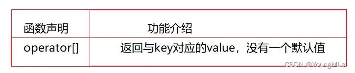
5. unordered_maps 实现了直接访问操作符 (operator[])，它允许使用 key 作为参数直接访问 value.
6. 它的迭代器至少是前向迭代器；

• unordered_map 的接口说明：

1. unordered_map 的容量接口：

2. unordered_map 的迭代器：

3. unordered_map 的元素访问：

4. unordered_map 的查询：

5. unordered_map 的修改操作

6. unordered_map 的桶操作

unordered_map 的简单使用如下，统计水果的个数：

		int main()
		{
			string arr[] = { "香蕉", "哈密瓜","苹果", "西瓜", "橙子", "西瓜", "苹果", "苹果", "西瓜", "橙子", "香蕉", "苹果", "香蕉" };
		
			unordered_map<string, int> hash;
		
			for (auto& str : arr)
			{
				hash[str]++;
			}
		
			unordered_map<string, int>::iterator it = hash.begin();
			while (it != hash.end())
			{
				cout << it->first << ":" << it->second << endl;
				++it;
			}
		
			return 0;
		}

统计结果如下：

3. unordered_set

unordered_set 的用法和接口都和 unordered_map 的类似，所以大家可以参考 unordered_map 的用法；下面可以参考 unordered_set 的文档介绍：unordered_set .

下面是 unordered_set 的简单使用：

		int main()
		{
			unordered_set<int> us;
			us.insert(10);
			us.insert(12);
			us.insert(92);
			us.insert(33);
		
			unordered_set<int>::iterator it = us.begin();
			while (it != us.end())
			{
				cout << *it << " ";
				++it;
			}
			cout << endl;
		
			for (auto e : us)
			{
				cout << e << " ";
			}
			cout << endl;
		
			return 0;
		}

结果如下：

二、底层结构

1. 哈希概念

unordered 系列的关联式容器之所以效率比较高，是因为其底层使用了哈希结构/哈希算法；

什么是哈希算法呢？哈希又称散列，本质就是映射，关键字与另一个值建立一个关联关系。

而 unordered_map 和 unordered_set 的底层是使用了哈希表，哈希表就是使用的哈希算法建立映射关系，将关键字和存储位置建立一个关联关系。

2. 哈希冲突

对于不同关键字通过相同哈希函数计算出相同的哈希地址，该种现象称为哈希冲突或哈希碰撞。

3. 哈希函数

哈希函数是通过关键字计算出该关键字的哈希地址的函数，常见的哈希函数有：直接定址法、除留余数法。

直接定址法：关键字和存储位置是一对一的关系，不存在哈希冲突；适用于关键字范围集中，数据量不大的情况。

除留余数法：关键字和存储位置是多对一的关系，存在哈希冲突；适用于关键字分散，数据量大的情况。

4. 解决哈希冲突

解决哈希冲突的两种常见方法是：闭散列和开散列。

（1）闭散列

闭散列：也叫开放定址法，当发生哈希冲突时，如果哈希表未被装满，说明在哈希表中必然还有空位置，那么可以把 key 存放到冲突位置中的下一个空位置中去；那如何寻找下一个空位置呢？

1. 线性探测

例如下图中，现在需要插入元素 44，先通过哈希函数计算哈希地址，hashAddr 为4，因此 44 理论上应该插在该位置，但是该位置已经放了值为4 的元素，即发生哈希冲突。

线性探测：从发生冲突的位置开始，依次向后探测，直到寻找到下一个空位置为止。

• 插入：通过哈希函数获取待插入元素在哈希表中的位置；如果该位置中没有元素则直接插入新元素，如果该位置中有元素发生哈希冲突，使用线性探测找到下一个空位置，插入新元素。

• 删除：采用闭散列处理哈希冲突时，不能随便物理删除哈希表中已有的元素，若直接删除元素会影响其他元素的搜索。比如删除元素 4，如果直接删除掉，44查找起来可能会受影响。因此线性探测采用标记的伪删除法来删除一个元素；例如我们可以像下面的代码这样实现：

    			// 哈希表每个空间给个标记
    			// EMPTY此位置空， EXIST此位置已经有元素， DELETE元素已经删除
    			enum State
    			{
    				EMPTY, 
    				EXIST, 
    				DELETE
    			};
  

下面我们开始用代码实现线性探测：

我们将线性探测的实现放入 open_address 的命名空间中，其中我们先实现每个数据的状态表示 Status，和每个数据的类型：

			namespace open_address
			{
				enum Status
				{
					EMPTY,
					EXIST,
					DELETE
				};
				
				template<class K, class V>
				struct HashData
				{
					pair<K, V> _kv;
					Status _status;
				};
			}

当 key 值为 string 类型或者其他类型的时候，我们没办法计算出它的哈希地址的位置，因此我们需要写仿函数来计算它特定的数据来获得哈希地址；当数据类型可以转成 size_t 或者类型是 string 的时候，可以通过以下两个仿函数转成 size_t 的类型，从而计算出哈希地址；代码如下：

			template<class K>
			class HashFunc
			{
			public:
				size_t operator()(const K& key)
				{
					return (size_t)key;
				}
			};
			
			template<>
			class HashFunc<string>
			{
			public:
				size_t operator()(const string& str)
				{
					size_t hashcnt = 0;
					for (auto e : str)
					{
						hashcnt *= 31;
						hashcnt += e;
					}
					return hashcnt;
				}
			};

下面我们引入一个概念：负载因子。负载因子是衡量表中的有效数据个数的表现，负载因子 = 存储数据的个数 / 表的大小；当负载因子达到一定程度的时候，表就需要扩容。

有了以上的铺垫就可以实现线性探测的代码了，代码如下：

			template<class K, class V, class Hash = HashFunc<K>>
			class HashTable
			{
			public:
				HashTable()
				{
					_tables.resize(10);
				}
		
				bool Insert(const pair<K, V>& kv)
				{
					if (Find(kv.first))
						return false;
		
					// 负载因子到 0.7 就扩容
					if (_n * 10 / _tables.size() == 7)
					{
						HashTable<K, V> NewTables;
						NewTables._tables.resize(_tables.size() * 2);
		
						// 将数据重新映射到新表上
						for (size_t i = 0; i < _tables.size(); i++)
						{
							if (_tables[i]._status == EXIST)
							{
								NewTables.Insert(_tables[i]._kv);
							}
						}
						// 新表和旧表的数据交换
						_tables.swap(NewTables._tables);
					}
					
					// 定义一个 Hash 的对象获取 kv.first 的 size_t 数据
					Hash hf;
					size_t hashi = hf(kv.first) % _tables.size();
					while (_tables[hashi]._status == EXIST)
					{
						++hashi;
		
						hashi %= _tables.size();
					}
		
					_tables[hashi]._kv = kv;
					_tables[hashi]._status = EXIST;
					++_n;
		
					return true;
				}
		
		
				HashData<K, V>* Find(const K& key)
				{
					Hash hf;
					size_t hashi = hf(key) % _tables.size();
					while (_tables[hashi]._status != EMPTY)
					{
						if (_tables[hashi]._status == EXIST
							&& _tables[hashi]._kv.first == key)
						{
							return &_tables[hashi];
						}
		
						++hashi;
						hashi %= _tables.size();
					}
					return nullptr;
				}
		
				bool Erase(const K& key)
				{
					// HashData<K, V>* del
					auto del = Find(key);
					if (del)
					{
						del->_status = DELETE;
						--_n;
						return true;
					}
					else
					{
						return false;
					}
				}
		
				void Print()
				{
					for (size_t i = 0; i < _tables.size(); i++)
					{
						if (_tables[i]._status == EXIST)
						{
							cout << "[" << i << "]->" << _tables[i]._kv.first << ":" << _tables[i]._kv.second << endl;
						}
						else if (_tables[i]._status == EMPTY)
						{
							printf("[%d]->\n", i);
						}
						else
						{
							printf("[%d]->DELETE\n", i);
						}
					}
					cout << endl;
				}
			
			// 实质是在顺序表上操作，所以哈希表可以用 vector
			private:
				vector<HashData<K, V>> _tables;
				size_t _n = 0;
			};

• 线性探测优点：实现非常简单，
• 线性探测缺点：一旦发生哈希冲突，所有的冲突连在一起，容易产生数据“堆积”，即：不同关键字占据了可利用的空位置，使得寻找某关键码的位置需要许多次比较，导致搜索效率降低。

（2）开散列

开散列概念：开散列法又叫链地址法(开链法)，首先对关键字集合用散列函数计算散列地址，具有相同地址的关键字归于同一个子集合，每一个子集合称为一个桶，各个桶中的元素通过一个单链表链接起来，各链表的头结点存储在哈希表中。如下图所示：

从上图可以看出，开散列中每个桶中放的都是发生哈希冲突的元素。

有了闭散列的实现基础，我们实现开散列就简单了，代码如下：

		namespace hash_bucket
		{
			// 节点的类
			template<class K, class V>
			struct HashNode
			{
				HashNode(const pair<K, V>& kv)
					:_kv(kv)
					,_next(nullptr)
				{}
		
				pair<K, V> _kv;
				HashNode* _next;
			};
			
			// 哈希表类
			template<class K, class V, class Hash = HashFunc<K>>
			class HashTable
			{
				typedef HashNode<K, V> Node;
		
			public:
				HashTable()
				{
					_tables.resize(10);
				}
				
				// 因为节点是我们一个一个 new 出来的，所以析构函数需要我们自己 delete 节点
				~HashTable()
				{
					for (size_t i = 0; i < _tables.size(); i++)
					{
						Node* cur = _tables[i];
						while (cur)
						{
							Node* next = cur->_next;
							delete cur;
							cur = next;
						}
						_tables[i] = nullptr;
					}
				}
		
				bool Insert(const pair<K, V>& kv)
				{
					Hash ht;
		
					// 扩容
					if (_n == _tables.size())
					{
						vector<Node*> NewTable(_tables.size() * 2, nullptr);
						//NewTable.resize(_tables.size() * 2, nullptr); // ???
						
						for (size_t i = 0; i < _tables.size(); i++)
						{
							Node* cur = _tables[i];
							while (cur)
							{
								Node* next = cur->_next;
		
								// 挪动到新映射后的新表
								size_t hashi = ht(cur->_kv.first) % NewTable.size(); 
								cur->_next = NewTable[hashi];
								NewTable[hashi] = cur;
		
								cur = next;
							}
							_tables[i] = nullptr;
						}
						_tables.swap(NewTable);
					}
		
					size_t hashi = ht(kv.first) % _tables.size();
					Node* newnode = new Node(kv);
		
					// 头插
					newnode->_next = _tables[hashi];
					_tables[hashi] = newnode;
					++_n;
		
					return true;
				}
		
				Node* Find(const K& key)
				{
					Hash ht;
					size_t hashi = ht(key) % _tables.size();
					Node* cur = _tables[hashi];
		
					while (cur)
					{
						if (cur->_kv.first == key)
						{
							return cur;
						}
						cur = cur->_next;
					}
					return nullptr;
				}
		
				bool Erase(const K& key)
				{
					Hash ht;
					size_t hashi = ht(key) % _tables.size();
					Node* prev = nullptr, * cur = _tables[hashi];
					while (cur)
					{
						if (cur->_kv.first == key)
						{
							if (prev == nullptr)
							{
								_tables[hashi] = cur;
							}
							else
							{
								prev->_next = cur->_next;
							}
							delete cur;
							return true;
						}
		
						prev = cur;
						cur = cur->_next;
					}
					return false;
				}
		
			private:
				vector<Node*> _tables;
				size_t _n = 0;
			};
		}

三、封装哈希表

1. 模板参数列表的改造

		template<class K, class T, class KeyOfT, class Hash = HashFunc<K>>
		class HashTable

• K：关键字类型；
• T：不同容器 T 的类型不同，如果是 unordered_map，V代表一个键值对，如果是 unordered_set，T 为 K；
• KeyOfT: 因为 T 的类型不同，通过 value 取 key 的方式就不同；
• Hash：哈希函数仿函数对象类型，哈希函数使用除留余数法，需要将 Key转换为整形数字才能取模；

2. 迭代器

			// 前置声明；为了实现简单，在哈希桶的迭代器类中需要用到 HashTable 本身，所以需要前置声明
			template<class K, class T, class KeyOfT, class Hash>
			class HashTable;
		
			template<class K, class T, class Ref, class Ptr, class KeyOfT, class Hash>
			struct __Iterator
			{
				typedef HashNode<T> Node;
				typedef __Iterator<K, T, Ref, Ptr, KeyOfT, Hash> Self;
		
				Node* _node;                                 // 当前迭代器关联的节点
				const HashTable<K, T, KeyOfT, Hash>* _pht;   // 哈希表桶，主要是为了找下一个空桶时候方便
				size_t _hashi;			                     // 当前哈希桶的位置
		
				__Iterator(Node* node, HashTable<K, T, KeyOfT, Hash>* pht, size_t hashi)
					:_node(node)
					,_pht(pht)
					,_hashi(hashi)
				{}
		
				__Iterator(Node* node, const HashTable<K, T, KeyOfT, Hash>* pht, size_t hashi)
					:_node(node)
					, _pht(pht)
					, _hashi(hashi)
				{}
				
				Self& operator++()
				{
					// 当前桶还有节点，走到下一个节点
					if (_node->_next)
					{
						_node = _node->_next;
					}
		
					// 当前桶已经走完了，找下一个不为空的桶
					else
					{
						// 走到下一个桶
						++_hashi;
						while (_hashi < _pht->_tables.size())
						{
							// 如果当前桶不为空，就将当前桶的指针给 _node
							if (_pht->_tables[_hashi])
							{
								_node = _pht->_tables[_hashi];
								break;
							}
							++_hashi;
						}
		
						// 如果遍历完所有桶，说明桶里面全是空，返回 nullptr
						if (_hashi == _pht->_tables.size())
						{
							_node = nullptr;
						}
					}
					return *this;
				}
		
				Ref operator*()
				{
					return _node->_data;
				}
		
				Ptr operator->()
				{
					return &_node->_data;
				}
		
				bool operator!=(const Self& s)
				{
					return _node != s._node;
				}
			};

3. HashTable 改造

			template<class K, class T, class KeyOfT, class Hash = HashFunc<K>>
			class HashTable
			{
				typedef HashNode<T> Node;
		
				// 让 __Iterator 成为友元
				template<class K, class T, class Ref, class Ptr, class KeyOfT, class Hash>
				friend struct __Iterator;
		
			public:
				typedef __Iterator<K, T, T&, T*, KeyOfT, Hash> iterator;
				typedef __Iterator<K, T, const T&, const T*, KeyOfT, Hash> const_iterator;
		
				iterator begin()
				{
					for (size_t i = 0; i < _tables.size(); i++)
					{
						if (_tables[i])
						{
							return iterator(_tables[i], this, i);
						}
					}
					return end();
				}
		
				iterator end()
				{
					return iterator(nullptr, this, -1);
				}
		
				const_iterator begin() const
				{
					for (size_t i = 0; i < _tables.size(); i++)
					{
						if (_tables[i])
						{
							return const_iterator(_tables[i], this, i);
						}
					}
					return end();
				}
		
				const_iterator end() const
				{
					return const_iterator(nullptr, this, -1);
				}
		
				HashTable()
				{
					_tables.resize(10);
				}
		
				~HashTable()
				{
					for (size_t i = 0; i < _tables.size(); i++)
					{
						Node* cur = _tables[i];
						while (cur)
						{
							Node* next = cur->_next;
							delete cur;
							cur = next;
						}
						_tables[i] = nullptr;
					}
				}
		
				pair<iterator, bool> Insert(const T& data)
				{
					Hash ht;
					KeyOfT kot;
		
					auto rit = Find(kot(data));
					if (rit !=	end())
						return make_pair(rit, false);
		
					// 扩容
					if (_n == _tables.size())
					{
						vector<Node*> NewTable(_tables.size() * 2, nullptr);
						//NewTable.resize(_tables.size() * 2, nullptr); // ???
						
						for (size_t i = 0; i < _tables.size(); i++)
						{
							Node* cur = _tables[i];
							while (cur)
							{
								Node* next = cur->_next;
		
								// 挪动到新映射后的新表
								size_t hashi = ht(kot(cur->_data)) % NewTable.size();
								cur->_next = NewTable[hashi];
								NewTable[hashi] = cur;
		
								cur = next;
							}
							_tables[i] = nullptr;
						}
						_tables.swap(NewTable);
					}
		
					size_t hashi = ht(kot(data)) % _tables.size();
					Node* newnode = new Node(data);
		
					// 头插
					newnode->_next = _tables[hashi];
					_tables[hashi] = newnode;
					++_n;
		
					return make_pair(iterator(newnode, this, hashi), true);
				}
		
				iterator Find(const K& key)
				{
					Hash ht;
					KeyOfT kot;
		
					size_t hashi = ht(key) % _tables.size();
					Node* cur = _tables[hashi];
		
					while (cur)
					{
						if (kot(cur->_data) == key)
						{
							return iterator(cur, this, hashi);
						}
						cur = cur->_next;
					}
					return end();
				}
		
				bool Erase(const K& key)
				{
					Hash ht;
					KeyOfT kot;
		
					size_t hashi = ht(kot(key)) % _tables.size();
					Node* prev = nullptr, * cur = _tables[hashi];
					while (cur)
					{
						if (cur->_kv.first == key)
						{
							if (prev == nullptr)
							{
								_tables[hashi] = cur;
							}
							else
							{
								prev->_next = cur->_next;
							}
							delete cur;
							return true;
						}
		
						prev = cur;
						cur = cur->_next;
					}
					return false;
				}
		
			private:
				vector<Node*> _tables;
				size_t _n = 0;
			};

4. my_unordered_map

			#pragma once
			
			#include "HashTable.h"
			
			
			template<class K, class V, class Hash = HashFunc<K>>
			class my_unordered_map
			{
				struct MapOfKey
				{
					const K& operator()(const pair<K, V>& kv)
					{
						return kv.first;
					}
				};
			
			public:
				typedef typename hash_bucket::HashTable<K, pair<const K, V>, MapOfKey, Hash>::iterator iterator;
				typedef typename hash_bucket::HashTable<K, pair<const K, V>, MapOfKey, Hash>::const_iterator const_iterator;
			
				iterator begin()
				{
					return _ht.begin();
				}
			
				iterator end()
				{
					return _ht.end();
				}
			
				const_iterator begin() const
				{
					return _ht.begin();
				}
			
				const_iterator end() const
				{
					return _ht.end();
				}
			
				pair<iterator, bool> insert(const pair<K, V>& kv)
				{
					return _ht.Insert(kv);
				}
			
				const V& operator[](const K& key) const
				{
					pair<iterator, bool> ret = _ht.Insert(make_pair(key, V()));
					return ret.first->second;
				}
			
				V& operator[](const K& key)
				{
					pair<iterator, bool> ret = _ht.Insert(make_pair(key, V()));
					return ret.first->second;
				}
			
				iterator find(const K& key)
				{
					return _ht.Find(key);
				}
			
				bool erase(const K& key)
				{
					return _ht.Erase(key);
				}
			
			private:
				hash_bucket::HashTable<K, pair<const K, V>, MapOfKey, Hash> _ht;
			};

5. my_unordered_set

			#pragma once
			#include "HashTable.h"
			
			
			template<class K, class Hash = HashFunc<K>>
			class my_unordered_set
			{
				struct SetOfKey
				{
					const K& operator()(const K& key)
					{
						return key;
					}
				};
			
			public:
			
				typedef typename hash_bucket::HashTable<K, K, SetOfKey, Hash>::const_iterator iterator;
				typedef typename hash_bucket::HashTable<K, K, SetOfKey, Hash>::const_iterator const_iterator;
			
				const_iterator begin() const
				{
					return _ht.begin();
				}
			
				const_iterator end() const
				{
					return _ht.end();
				}
			
				pair<const_iterator, bool> insert(const K& key)
				{
					auto ret = _ht.Insert(key);
					return pair<const_iterator, bool>(const_iterator(ret.first._node, ret.first._pht, ret.first._hashi), ret.second);
				}
			
				iterator find(const K& key)
				{
					return _ht.Find(key);
				}
			
				bool erase(const K& key)
				{
					return _ht.Erase(key);
				}
			private:
				hash_bucket::HashTable<K, K, SetOfKey, Hash> _ht;
			};

四、哈希的应用

1. 位图

• 位图概念

所谓位图，就是用每一位来存放某种状态，适用于海量数据，数据无重复的场景。通常是用来判断某个数据存不存在的。

我们先来看一下下面这道题：给40亿个不重复的无符号整数，没排过序。给一个无符号整数，如何快速判断一个数是否在这40亿个数中？

首先我们能想到的是遍历一遍，但是这样的时间复杂度是 O(N) ，而且内存也开不出这么大的连续空间去存放这些数；首先每个整型是 4 个 byte，这里需要 40 亿个整型单位，也就是 160 亿个 byte，也就是 14 G 左右，不符合实际情况。

第二种我们能想到的是二分查找，但是二分查找的前提是有序，而排序的代价更大，而且也会同时面临第一种方法的内存问题，也不符合实际。

最后我们可以考虑用一个比特位来标记某一个数是否出现过，这就是最后一个方法解决：位图；也就是每个值映射一个比特位，此时我们只需要 0.5G 左右的内存，如下图所示：

那么我们要怎样计算某一个数在数组中的哪一个整型中呢？因为每个整型 32 个 bit 位，所以我们设某一个数为 x，想要知道它在数组的哪一个整型，可以用 i = x / 32，i 就是 x 在数组中的第 i 整型中。

那么又怎么计算 x 在这个整型的第几位呢？我们可以用 j = x % 32 得到，也就是 x 除以 32 的余数。

下面我们简单实现一下位图，只需要用到简单的位运算即可，代码如下：

		template<size_t N>
		class bit_set
		{
		public:
			bit_set()
			{
				_bits.resize(N / 32 + 1, 0);
			}
		
			void set(size_t x)
			{
				size_t i = x / 32;
				size_t j = x % 32;
				_bits[i] |= (1 << j);
			}
		
			void reset(size_t x)
			{
				size_t i = x / 32;
				size_t j = x % 32;
				_bits[i] &= ~(1 << j);
			}
		
			bool test(size_t x)
			{
				size_t i = x / 32;
				size_t j = x % 32;
				return _bits[i] & (1 << j);
			}
			
		private:
			vector<int> _bits;
		};

其中 set 是将 x 在 _bits 中映射的比特位设置为 1，即标记为出现过；reset 则相反，将标记为设为 0；test 则是返回 x 映射的比特位的情况，即判断这个位是 1 还是 0，1 即存在，0 即不存在。

下面我们看另外一个问题：给两个文件，分别有100亿个整数，只有1G内存，如何找到两个文件交集？

此时我们就可以各自映射到一个位图，一个值在两个位图都存在，则是交集。

最后我们看一个位图应用变形问题：1个文件有100亿个int，1G内存，设计算法找到出现次数不超过2次的所有整数？

此时我们的每个位置应该需要表示四种状态：出现 0 次、出现 1 次、出现 2 次、出现 3 次及以上；所以我们可以考虑用两个 bit_set 表示两个比特位从而表示该状态，出现 0 次：00；出现 1 次：01；出现 2 次：10；出现 3 次及以上：11；下面我们用代码实现：

		template<size_t N>
		class twobitset
		{
		public:
			void set(size_t x)
			{
				// 00 -> 01
				// 01 -> 10
				// 10 -> 11
				// 11 -> 不变
				if (_bs1.test(x) == false && _bs2.test(x) == false)
				{
					_bs2.set(x);
				}
				else if (_bs1.test(x) == false && _bs2.test(x) == true)
				{
					_bs1.set(x);
					_bs2.reset(x);
				}
				else if (_bs1.test(x) == true && _bs2.test(x) == false)
				{
					_bs1.set(x);
					_bs2.set(x);
				}
			}
		
			// 打印出出现次数不超过两次的整数
			void Print()
			{
				for (size_t i = 0; i < N; i++)
				{
					if (_bs1.test(i) == false && _bs2.test(i) == true)
					{
						cout << "1->" << i << endl;
					}
					else if (_bs1.test(i) == true && _bs2.test(i) == false)
					{
						cout << "2->" << i << endl;
					}
				}
				cout << endl;
			}
		
		private:
			bit_set<N> _bs1;
			bit_set<N> _bs2;
		};

2. 布隆过滤器

我们学了上面的哈希和位图，可以对它们进行总结：

1. 用哈希表存储用户记录，缺点：浪费空间；
2. 用位图存储用户记录，缺点：位图一般只能处理整形，如果内容编号是字符串，就无法处理了；
3. 将哈希与位图结合，即布隆过滤器。

布隆过滤器概念：布隆过滤器是由布隆（Burton Howard Bloom）在1970年提出的 一种紧凑型的、比较巧妙的概率型数据结构，特点是高效地插入和查询，可以用来告诉你 “某样东西一定不存在或者可能存在”，它是用多个哈希函数，将一个数据映射到位图结构中。此种方式不仅可以提升查询效率，也可以节省大量的内存空间。

以字符串为类型，例如下图的映射关系：

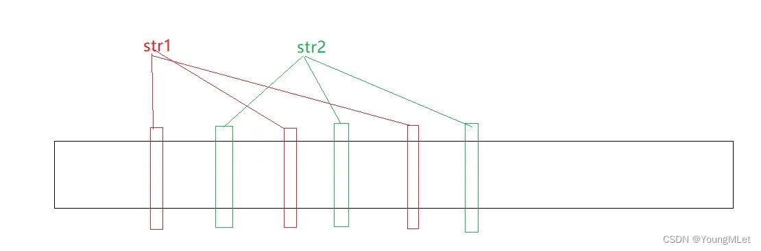
其中 str1 用三种不同的哈希函数计算出不同的整型值，对应映射三个不同的比特位，但是还是可能存在冲突(误判)。布隆过滤器特点是为了节省空间，映射位越多，消耗的空间就越多。

那么我们继续以字符串为类型，判断一个字符串在不在，到底是这个字符串在准确，还是这个字符串不在准确呢？

例如上图，str3 映射的位置与 str1 和 str2 都有重叠的映射比特位，那么如果我们单纯判断 bitset1 和 bitset2 就得出结果 str3 存在，准确吗？答案是不准确的！因为 str3 还有一个映射位置 bitset3，只有三个位置同时为 1，str3 才是存在的！但是只要有一个位置是 0，那么就说明某个字符串不存在。所以我们得出结论：判断某个字符串是否存在，在：是不准确的；不在：是准确的。

下面我们用代码简单实现一下布隆过滤器：

由于我们需要使用位图，所以在头文件先包含我们上面实现的位图的头文件：#include "bit_set.h"

接下来设计三种不同的哈希函数：

		// 1、BKDRHash
		struct BKDRHash
		{
			size_t operator()(const string& key)
			{
				// BKDR
				size_t hash = 0;
				for (auto e : key)
				{
					hash *= 31;
					hash += e;
				}
		
				return hash;
			}
		};
		
		
		// 2、APHash
		struct APHash
		{
			size_t operator()(const string& key)
			{
				size_t hash = 0;
				for (size_t i = 0; i < key.size(); i++)
				{
					char ch = key[i];
					if ((i & 1) == 0)
					{
						hash ^= ((hash << 7) ^ ch ^ (hash >> 3));
					}
					else
					{
						hash ^= (~((hash << 11) ^ ch ^ (hash >> 5)));
					}
				}
				return hash;
			}
		};
		
		
		// 3、DJBHash
		struct DJBHash
		{
			size_t operator()(const string& key)
			{
				size_t hash = 5381;
				for (auto ch : key)
				{
					hash += (hash << 5) + ch;
				}
				return hash;
			}
		};

接下来是布隆过滤器的实现，模板参数我们默认以 string 为缺省参数，然后是三种不同的哈希函数：

		template <size_t N, class K = string, 
			class HashFunc1 = BKDRHash,
			class HashFunc2 = APHash,
			class HashFunc3 = DJBHash>
		class BloomFilter
		{
		public:
			void set(const K& key)
			{
				size_t hash1 = HashFunc1()(key) % N;
				size_t hash2 = HashFunc2()(key) % N;
				size_t hash3 = HashFunc3()(key) % N;
		
				_bs.set(hash1);
				_bs.set(hash2);
				_bs.set(hash3);
			}
		
			// 一般不支持删除，因为删除一个值可能会影响其他值
			// void reset(const K& key);
		
			bool test(const K& key)
			{
				// 判断不在是准确的
				size_t hash1 = HashFunc1()(key) % N;
				if (_bs.test(hash1) == false)
					return false;
		
				size_t hash2 = HashFunc2()(key) % N;
				if (_bs.test(hash2) == false)
					return false;
		
				size_t hash3 = HashFunc3()(key) % N;
				if (_bs.test(hash3) == false)
					return false;
		
				// 存在误判
				return true;
			}
		
		private:
			bit_set<N> _bs;
		};

下面我们简单测试一下：

		int main()
		{
			BloomFilter<50> bf;
			bf.set("aaaaa");
			bf.set("bbbbb");
			bf.set("ccccc");
		
			cout << bf.test("aaaaa") << endl;
			cout << bf.test("bbbbb") << endl;
			cout << bf.test("ccccc") << endl;
			cout << bf.test("aaabb") << endl;
		
		
			return 0;
		}

结果如下：

布隆过滤器优点：

1. 增加和查询元素的时间复杂度为:O(K), (K为哈希函数的个数，一般比较小)，与数据量大小无关；
2. 哈希函数相互之间没有关系，方便硬件并行运算；
3. 布隆过滤器不需要存储元素本身，在某些对保密要求比较严格的场合有很大优势；
4. 在能够承受一定的误判时，布隆过滤器比其他数据结构有这很大的空间优势；
5. 数据量很大时，布隆过滤器可以表示全集，其他数据结构不能；
6. 使用同一组散列函数的布隆过滤器可以进行交、并、差运算。

布隆过滤器缺陷：

1. 有误判率，即存在假阳性(False Position)，即不能准确判断元素是否在集合中(补救方法：再建立一个白名单，存储可能会误判的数据)；
2. 不能获取元素本身；
3. 一般情况下不能从布隆过滤器中删除元素；
4. 如果采用计数方式删除，可能会存在计数回绕问题；