写在前面
参考的是https://zh.d2l.ai/index.html
一、大作业设计目的与要求
(1)利用所学习的聚类算法完成简单的图像分割系统。
(2)编程并利用相关软件完成大作业测试,得到实验结果。
(3)通过对实验结果的分析得出实验结论,培养学生创新思维和编写实验报告的能力,以及处理一般工程设计技术问题的初步能力及实事求是的科学态度。
(4)利用实验更加直观、方便和易于操作的优势,提高学生学习兴趣,让学生自主发挥设计和实施实验,发挥出学生潜在的积极性和创造性。
(5)通过实验的锻炼,使学生进一步掌握基于卷积神经网络的图像分类问题,也进一步领会学习机器学习知识的重要意义。
二、大作业设计内容
大作业1 :手写数字识别系统。
本项目要求选择机器学习算法设计实现手写数字识别系统。手写数字识别在日常生活中有重要应用,例如汇款单、银行支票的处理,以及邮件的分拣等。手写数字识别通常对精度要求较高,虽然只有10类,但是每个人的字迹不同,要做到精确识别有一定难度。项目的具体要求如下:
(1)使用MNIST手写数字数据集,进行手写数字识别(参考课本P186, 例6.2 )。
(2)选择合适的机器学习算法进行手写数字识别,训练分类模型,要求识别精度尽可能高。
(3)编写简单用户界面,可以加载手写数字图片,并调用算法识别数字。
三、程序开发与运行环境
显卡:NVIDIA显卡,CUDA 11.7。
系统与环境:Windows11操作系统,Anaconda3的base虚拟环境。
IDE:Pycharm Community集成开发环境,Jupyter Notebook
深度学习框架:PyTorch深度学习框架,基于GPU版本。
图形界面框架:PyQt5
四、设计正文
(包括分析与设计思路、各模块流程图、主要算法伪代码等,如有改进或者拓展,请重点用一小节进行说明)
4.1 分析与设计思路与流程图
本次实验任务是使用MNIST手写数据集进行手写数字识别。使用传统的多层感知机等神经网络模型不能很好地解决此类问题,因为这种模型直接读取图像的原始像素,基于图像的原始像素进行分类。然而,图像特征的提取还需要人工设计函数进行提取。所以,卷积神经网络模型可以很好地对图像进行自动的特征提取。
本次大作业使用经典的AlexNet卷积神经网络模型。AlexNet卷积神经网络模型具有以下整体结构:
包含8层变换,包括5层卷积和2层全连接的隐藏层,1个全连接的输出层。其中,第一层的卷积窗口形状为1111,可以支持输入更大的图像。第二层卷积窗口形状减小到55,之后的3层卷积采用33的窗口。在第一、第二、第五个卷积层之后都使用了卷积窗口大小为33、且步幅为2的最大池化。卷积通道数比LeNet大了10倍。在最后一个卷积与池化层后,就是两个输出个数为4096的全连接层,最后输出结果。
1.引入了图像增广、翻转、裁剪等方法,进一步从原始数据集中制作、扩大数据集。
AlexNet流程图如下:
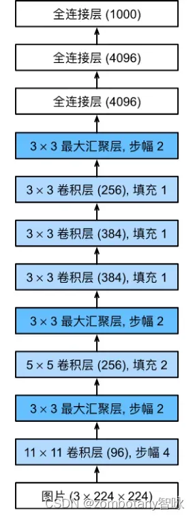
在本实验中,因为运行的是MNIST数据集,所以最后一个全连接层只有10个结点,而非该流程图中的1000。
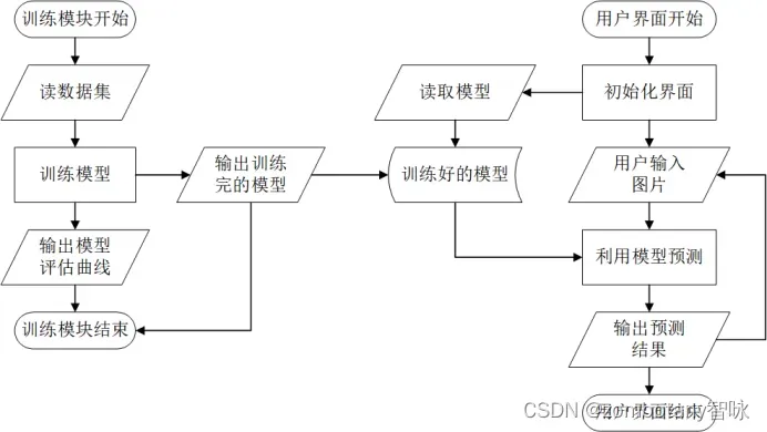
为了进行图形化的界面展示,还利用PyQt框架设置了前端图形界面。
在训练完成数据集后,将模型写入硬盘文件并保存,以供前端的图形界面调用、读取。
所以,前端的图形界面在初始化过程中,就预先加载好了训练好的模型。用户可以从文件中读入需要识别的手写数字图片,由前端图形界面根据加载好的模型自动给出该手写数字图片的识别结果。所以,本次实验中各个模块的交互逻辑如下图所示。
4.2 主要算法代码
训练模型
import numpy as np  # numpy数组库
import math  # 数学运算库
import matplotlib.pyplot as plt  # 画图库
import torch  # torch基础库
import torchvision.datasets as dataset  # 公开数据集的下载和管理
import torchvision.transforms as transforms  # 公开数据集的预处理库,格式转换
import torchvision.utils as utils
import torch.utils.data as data_utils  # 对数据集进行分批加载的工具集
from torch.utils import data
from d2l import torch as d2l
d2l.use_svg_display()
from torch import nn
net = nn.Sequential(
    # 这里,我们使用一个11*11的更大窗口来捕捉对象。
    # 同时,步幅为4,以减少输出的高度和宽度。
    # 另外,输出通道的数目远大于LeNet
    nn.Conv2d(1, 96, kernel_size=11, stride=4, padding=1), nn.ReLU(),
    nn.MaxPool2d(kernel_size=3, stride=2),
    # 减小卷积窗口,使用填充为2来使得输入与输出的高和宽一致,且增大输出通道数
    nn.Conv2d(96, 256, kernel_size=5, padding=2), nn.ReLU(),
    nn.MaxPool2d(kernel_size=3, stride=2),
    # 使用三个连续的卷积层和较小的卷积窗口。
    # 除了最后的卷积层,输出通道的数量进一步增加。
    # 在前两个卷积层之后,汇聚层不用于减少输入的高度和宽度
    nn.Conv2d(256, 384, kernel_size=3, padding=1), nn.ReLU(),
    nn.Conv2d(384, 384, kernel_size=3, padding=1), nn.ReLU(),
    nn.Conv2d(384, 256, kernel_size=3, padding=1), nn.ReLU(),
    nn.MaxPool2d(kernel_size=3, stride=2),
    nn.Flatten(),
    # 这里,全连接层的输出数量是LeNet中的好几倍。使用dropout层来减轻过拟合
    nn.Linear(6400, 4096), nn.ReLU(),
    nn.Dropout(p=0.5),
    nn.Linear(4096, 4096), nn.ReLU(),
    nn.Dropout(p=0.5),
    # 最后是输出层。由于这里使用MNIST,所以用类别数为10,而非论文中的1000
    nn.Linear(4096, 10))
X = torch.randn(1, 1, 224, 224)#随机初值
for layer in net:#用随机权重参数初始化CNN
    X=layer(X)
    print(layer.__class__.__name__,'output shape:\t',X.shape)
def load_data_mnist(batch_size, resize=None):#读取、加载MNIST数据集,并batch
    trans = [transforms.ToTensor()]
    if resize:
        trans.insert(0, transforms.Resize(resize))
    trans = transforms.Compose(trans)
    mnist_train = dataset.MNIST(
        root="../data", train=True, transform=trans, download=True)
    mnist_test = dataset.MNIST(
        root="../data", train=False, transform=trans, download=True)
    return (data.DataLoader(mnist_train, batch_size, shuffle=True,
                            num_workers=4),
            data.DataLoader(mnist_test, batch_size, shuffle=False,
                            num_workers=4))
batch_size = 128
train_iter, test_iter = load_data_mnist(batch_size=batch_size,resize=224)
for i, (X, y) in enumerate(train_iter):
    device = torch.device("cuda" if torch.cuda.is_available() else "cpu")
    X, y = X.to(device), y.to(device)
    print("X:",X.shape)
    print("y:",y.shape)
def evaluate_accuracy_gpu(net, data_iter, device=None): #@save
    """使用GPU计算模型在数据集上的精度"""
    if isinstance(net, nn.Module):
        net.eval()  # 设置为评估模式
        if not device:
            device = next(iter(net.parameters())).device
    # 正确预测的数量,总预测的数量
    metric = d2l.Accumulator(2)
    with torch.no_grad():
        for X, y in data_iter:
            if isinstance(X, list):
                # BERT微调所需的
                X = [x.to(device) for x in X]
            else:
                X = X.to(device)
            y = y.to(device)
            metric.add(d2l.accuracy(net(X), y), y.numel())
    return metric[0] / metric[1]
def train_ch6(net, train_iter, test_iter, num_epochs, lr, device):
    """用GPU训练模型(在第六章定义)"""
    def init_weights(m):
        if type(m) == nn.Linear or type(m) == nn.Conv2d:
            nn.init.xavier_uniform_(m.weight)
    net.apply(init_weights)
    print('training on', device)
    net.to(device)
    optimizer = torch.optim.SGD(net.parameters(), lr=lr)
    loss = nn.CrossEntropyLoss()
    animator = d2l.Animator(xlabel='epoch', xlim=[1, num_epochs],
                            legend=['train loss', 'train acc', 'test acc'])
    timer, num_batches = d2l.Timer(), len(train_iter)
    for epoch in range(num_epochs):
        # 训练损失之和,训练准确率之和,样本数
        metric = d2l.Accumulator(3)
        net.train()
        for i, (X, y) in enumerate(train_iter):
            timer.start()
            optimizer.zero_grad()
            X, y = X.to(device), y.to(device)
            y_hat = net(X)
            l = loss(y_hat, y)
            l.backward()
            optimizer.step()
            with torch.no_grad():
                metric.add(l * X.shape[0], d2l.accuracy(y_hat, y), X.shape[0])
            timer.stop()
            train_l = metric[0] / metric[2]
            train_acc = metric[1] / metric[2]
            if (i + 1) % (num_batches // 5) == 0 or i == num_batches - 1:
                animator.add(epoch + (i + 1) / num_batches,
                             (train_l, train_acc, None))
        test_acc = evaluate_accuracy_gpu(net, test_iter)
        animator.add(epoch + 1, (None, None, test_acc))
        animator.show()
    print(f'loss {train_l:.3f}, train acc {train_acc:.3f}, '
          f'test acc {test_acc:.3f}')
    print(f'{metric[2] * num_epochs / timer.sum():.1f} examples/sec '
          f'on {str(device)}')

lr, num_epochs = 0.01, 10
train_ch6(net, train_iter, test_iter, num_epochs, lr, d2l.try_gpu())

torch.save(net, "cnn.pt")
用户界面
from PIL import Image, ImageDraw, ImageFont
from PyQt5.QtWidgets import (QMainWindow, QMenuBar, QToolBar, QTextEdit, QAction, QApplication,
                             qApp, QMessageBox, QFileDialog, QLabel, QHBoxLayout, QGroupBox,
                             QComboBox, QGridLayout, QLineEdit, QSlider, QPushButton)
from PyQt5.QtGui import *
from PyQt5.QtGui import QPalette, QImage, QPixmap, QBrush
from PyQt5.QtCore import *
import sys
import cv2 as cv
import cv2
import numpy as np
import time
from pylab import *
import os
from torchvision import transforms
from PIL import Image
import torch
import numpy as np

class Window(QMainWindow):
    path = ' '
    change_path = "change.png"#被处理过的图像的路径
    IMG1 = ' '
    IMG2 = 'null'

    def __init__(self):
        super(Window, self).__init__()
        # 界面初始化

        self.createMenu()#创建左上角菜单栏
        self.cwd = os.getcwd()#当前工作目录
        self.image_show()
        self.label1 = QLabel(self)
        self.initUI()

    # 菜单栏
    def createMenu(self):
        # menubar = QMenuBar(self)
        menubar = self.menuBar()
        menu1 = menubar.addMenu("文件")
        menu1.addAction("打开")
        menu1.triggered[QAction].connect(self.menu1_process)

    #展示大图片
    def image_show(self):
        self.lbl = QLabel(self)
        self.lbl.setPixmap(QPixmap('source.png'))
        self.lbl.setAlignment(Qt.AlignCenter)  # 图像显示区,居中
        self.lbl.setGeometry(35, 35, 800, 700)
        self.lbl.setStyleSheet("border: 2px solid black")

    def initUI(self):
        self.setGeometry(50, 50, 900, 800)
        self.setWindowTitle('mnist识别系统')
        palette = QPalette()
        palette.setColor(self.backgroundRole(), QColor(255, 255, 255))
        self.setPalette(palette)

        self.label1.setText("TextLabel")
        self.label1.move(100,730)
        self.show()
    # 菜单1处理
    def menu1_process(self, q):
        self.path = QFileDialog.getOpenFileName(self, '打开文件', self.cwd,
                                                "All Files (*);;(*.bmp);;(*.tif);;(*.png);;(*.jpg)")
        self.image = cv.imread(self.path[0])
        self.lbl.setPixmap(QPixmap(self.path[0]))
        cv2.imwrite(self.change_path, self.image)
        transforms1 = transforms.Compose([
            transforms.ToTensor()
        ])
        self.label1.setText("识别中")
        img = Image.open(self.change_path)
        img = img.convert("L")
        img = img.resize((224, 224))
        tensor = transforms1(img)
        print(tensor.shape)
        tensor = tensor.type(torch.FloatTensor)
        device = torch.device("cuda" if torch.cuda.is_available() else "cpu")
        tensor = tensor.to(device)
        tensor = tensor.reshape((1, 1, 224, 224))
        print(tensor.shape)
        y = net(tensor)
        print(y)
        print(torch.argmax(y))
        self.label1.setText(str(int(torch.argmax(y))))
if __name__ == '__main__':
    net = torch.load('cnn.pt')
    app = QApplication(sys.argv)
    ex = Window()
    ex.show()
    sys.exit(app.exec_())
4.3 改进与拓展
1.重新配置了环境,安装了基于GPU版本的Pytorch。与CPU版本相比,GPU能够支持更快的卷积运算。同时,更大的显存也能够支持将更多的数据batch分批处理,有利于训练的稳定性防止“梯度消失”。在CPU版本中,若batch size过大则可能出现爆内存等问题。
2.AlexNet将sigmoid激活函数替换成了更简单的ReLU激活函数。ReLU的计算更简单,使得模型更容易训练,不会造成“梯度消失”等使得模型无法得到有效训练的情况。
3.为了防止过拟合,还引入了一定概率的dropout控制全连接层的模型复杂度。
五、实验运行结果及分析
(不同情形的运行结果及详细分析)
以下为python控制台输出结果
D:\ProgramData\Anaconda3\python.exe F:/mnist/mlhw3.py
Conv2d output shape: torch.Size([1, 96, 54, 54])
ReLU output shape: torch.Size([1, 96, 54, 54])
MaxPool2d output shape: torch.Size([1, 96, 26, 26])
Conv2d output shape: torch.Size([1, 256, 26, 26])
ReLU output shape: torch.Size([1, 256, 26, 26])
MaxPool2d output shape: torch.Size([1, 256, 12, 12])
Conv2d output shape: torch.Size([1, 384, 12, 12])
ReLU output shape: torch.Size([1, 384, 12, 12])
Conv2d output shape: torch.Size([1, 384, 12, 12])
ReLU output shape: torch.Size([1, 384, 12, 12])
Conv2d output shape: torch.Size([1, 256, 12, 12])
ReLU output shape: torch.Size([1, 256, 12, 12])
MaxPool2d output shape: torch.Size([1, 256, 5, 5])
Flatten output shape: torch.Size([1, 6400])
Linear output shape: torch.Size([1, 4096])
ReLU output shape: torch.Size([1, 4096])
Dropout output shape: torch.Size([1, 4096])
Linear output shape: torch.Size([1, 4096])
ReLU output shape: torch.Size([1, 4096])
Dropout output shape: torch.Size([1, 4096])
Linear output shape: torch.Size([1, 10])
training on cuda:0
<Figure size 350x250 with 1 Axes>
<Figure size 350x250 with 1 Axes>
<Figure size 350x250 with 1 Axes>
<Figure size 350x250 with 1 Axes>
<Figure size 350x250 with 1 Axes>
<Figure size 1920x951 with 1 Axes>
<Figure size 1920x951 with 1 Axes>
<Figure size 1920x951 with 1 Axes>
<Figure size 1920x951 with 1 Axes>
<Figure size 1920x951 with 1 Axes>
<Figure size 1920x951 with 1 Axes>
<Figure size 1920x951 with 1 Axes>
<Figure size 1920x951 with 1 Axes>
<Figure size 1920x951 with 1 Axes>
<Figure size 1920x951 with 1 Axes>
<Figure size 1920x951 with 1 Axes>
<Figure size 1920x951 with 1 Axes>
<Figure size 1920x951 with 1 Axes>
<Figure size 1920x951 with 1 Axes>
<Figure size 1920x951 with 1 Axes>
<Figure size 1920x951 with 1 Axes>
<Figure size 1920x951 with 1 Axes>
<Figure size 1920x951 with 1 Axes>
<Figure size 1920x951 with 1 Axes>
<Figure size 1920x951 with 1 Axes>
<Figure size 1920x951 with 1 Axes>
<Figure size 1920x951 with 1 Axes>
<Figure size 1920x951 with 1 Axes>
<Figure size 1920x951 with 1 Axes>
<Figure size 1920x951 with 1 Axes>
<Figure size 1920x951 with 1 Axes>
<Figure size 1920x951 with 1 Axes>
<Figure size 1920x951 with 1 Axes>
<Figure size 1920x951 with 1 Axes>
<Figure size 1920x951 with 1 Axes>
<Figure size 1920x951 with 1 Axes>
<Figure size 1920x951 with 1 Axes>
<Figure size 1920x951 with 1 Axes>
<Figure size 1920x951 with 1 Axes>
<Figure size 1920x951 with 1 Axes>
<Figure size 1920x951 with 1 Axes>
<Figure size 1920x951 with 1 Axes>
<Figure size 1920x951 with 1 Axes>
<Figure size 1920x951 with 1 Axes>
<Figure size 1920x951 with 1 Axes>
<Figure size 1920x951 with 1 Axes>
<Figure size 1920x951 with 1 Axes>
<Figure size 1920x951 with 1 Axes>
<Figure size 1920x951 with 1 Axes>
<Figure size 1920x951 with 1 Axes>
<Figure size 1920x951 with 1 Axes>
<Figure size 1920x951 with 1 Axes>
<Figure size 1920x951 with 1 Axes>
<Figure size 1920x951 with 1 Axes>
<Figure size 1920x951 with 1 Axes>
<Figure size 1920x951 with 1 Axes>
<Figure size 1920x951 with 1 Axes>
<Figure size 1920x951 with 1 Axes>
<Figure size 1920x951 with 1 Axes>
<Figure size 1920x951 with 1 Axes>
<Figure size 1920x951 with 1 Axes>
<Figure size 1920x951 with 1 Axes>
<Figure size 1920x951 with 1 Axes>
<Figure size 1920x951 with 1 Axes>
<Figure size 1920x951 with 1 Axes>
<Figure size 1920x951 with 1 Axes>
<Figure size 1920x951 with 1 Axes>
<Figure size 1920x951 with 1 Axes>
<Figure size 1920x951 with 1 Axes>
<Figure size 1920x951 with 1 Axes>
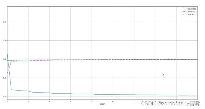
loss 0.039, train acc 0.988, test acc 0.991
624.4 examples/sec on cuda:0
可以看出,正确地建立了模型,正确地进行迭代与更新、训练的过程。训练完成后,loss函数为0.039,训练集准确率为0.988,测试集准确率为0.991。在cuda上,每一秒都运行了624个训练数据。
训练集准确率、测试集准确率、loss函数的变化曲线如下。可以看出,其识别精度是非常高的。
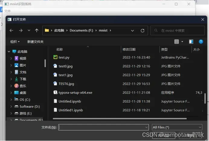
此为用户图形界面
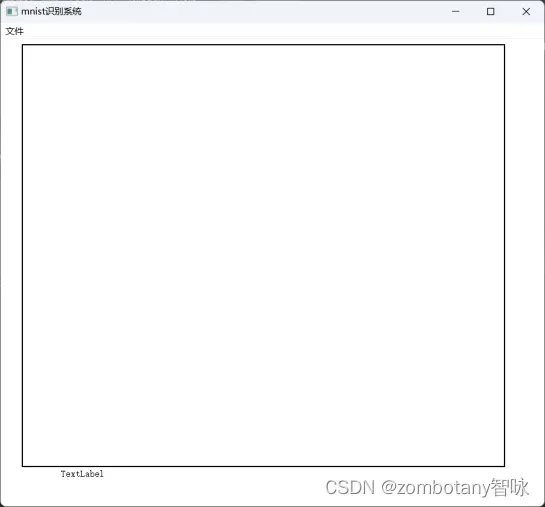
可以读取文件
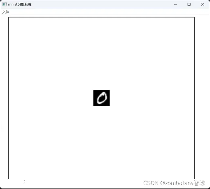
读取数字“0”的图片并正确识别。该图片为真实手写并反色处理后的图片,不来源于训练集。
控制台输出如下:
torch.Size([1, 224, 224])
torch.Size([1, 1, 224, 224])
tensor([[16.5969, -2.6974,  1.0315, -4.3109, -2.4112, -2.2494,  2.9837, -2.5753,
         -1.0474,  0.4374]], device='cuda:0', grad_fn=<AddmmBackward0>)
tensor(0, device='cuda:0')
用户界面如下:
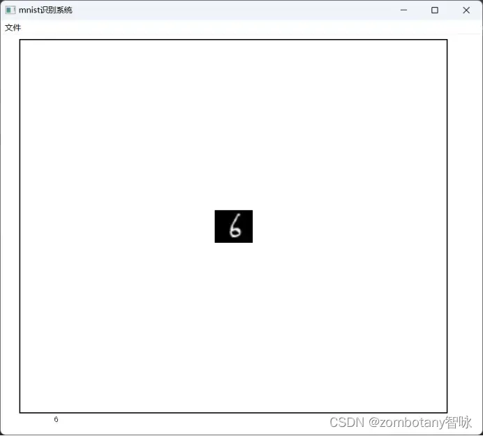
读取数字“6”并正确识别。该图片为真实手写并反色处理后的图片,不来源于训练集。
控制台输出如下:
torch.Size([1, 224, 224])
torch.Size([1, 1, 224, 224])
tensor([[-3.4247, -0.9304, -0.6991, -1.0964,  0.0769,  2.2364, 11.2306, -6.2827,
          6.0278, -7.4283]], device='cuda:0', grad_fn=<AddmmBackward0>)
tensor(6, device='cuda:0')
用户界面如下:
六、总结与进一步改进设想
在本次实验中,使用了经典的AlexNet卷积神经网络对经典的MNIST数据集进行训练。完成了模型搭建与训练的任务,识别精度也足够高,也编写了简单的用户界面,用真实手写的图片进行测试,可以看出模型对于真实场景的效果也是适用的,而不是只适用于加载出来并分割出来的测试集。
为了进一步改进,可以引入图像增广、翻转、裁剪、颜色变化等办法进一步扩大制作数据集,用于训练与测试。可以使用RGB颜色的3通道彩图而不是仅仅使用单通道二值化图像进行训练。
七、参考文献
[1]周志华. 机器学习[M]. 2016年1月第1版. 北京:清华大学出版社, 2016.
[2]赵卫东, 董亮. 机器学习[M]. 2018年8月第1版. 北京:人民邮电出版社, 2018.
[3]李航. 统计学习方法[M]. 2019年5月第2版. 北京:清华大学出版社, 2019.
[4]阿斯顿·张(Aston Zhang), 李沐(Mu Li), [美]扎卡里·C.立顿(Zachary C.Lipton), 等. 动手学深度学习[M]. 2019年6月第1版. 北京:人民邮电出版社, 2019.
[5][美]Ian Goodfellow [加]Yoshua Bengio [加]Aaron Courville. 深度学习[M]. 2017年8月第1版. 北京:人民邮电出版社, 2017.
文章出处登录后可见!