1. Rasterio与Rioxarray安装
Rasterio 是一个很多模块是基于 GDAL 的 Python 包,可用于处理地理空间栅格数据,例如 GeoTIFF 文件。为此,可以使用许多模块和函数,例如,处理来自卫星的原始数据、读取栅格数据、检索地理元数据、转换坐标、裁剪图像、合并多个图像以及以其他格式保存数据。大量的功能和易于实施使 Rasterio 成为卫星数据分析的标准工具。
首先安装 Rasterio 模块,(本人使用 conda 安装时遇到过报错 ImportError: cannot import name 'CRS' from 'pyproj' (unknown location),是由于 pyproj 模块安装不全,因此建议采用后面的离线安装方式或者之后遇到问题时删除 pyproj 模块后再离线安装该模块):
conda install gdal
conda install rasterio
如果安装失败可以采用离线安装的方式,Rasterio 依赖很多第三方库,所以比较麻烦,按下面的顺序依次安装即可,可以尝试使用 pip 安装或者下载 .whl 文件离线安装(注意对上 Python 版本):
pyproj
Shapely
GDAL
Fiona
rasterio
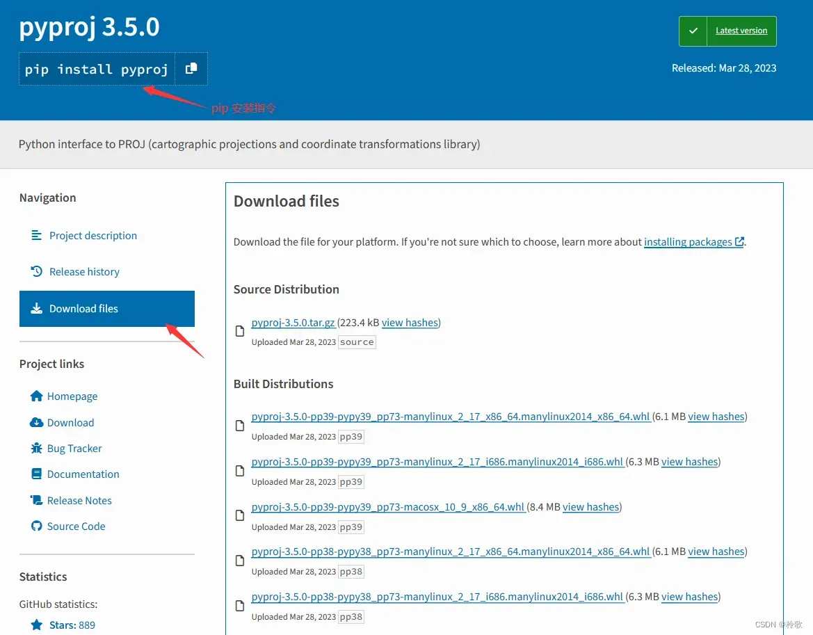
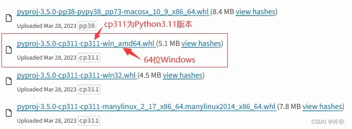
各个模块的链接:Pyproj、Shapely、GDAL、Fiona、Rasterio。
离线安装指令:
pip install E:\GDAL-1.2.10-cp310-cp310-win_amd64.whl
在 Python 中使用 Anaconda 安装 rioxarray 包时,首先需要安装 GDAL 和 rasterio,然后再安装 rioxarray:
pip install rioxarray
2. 使用教程
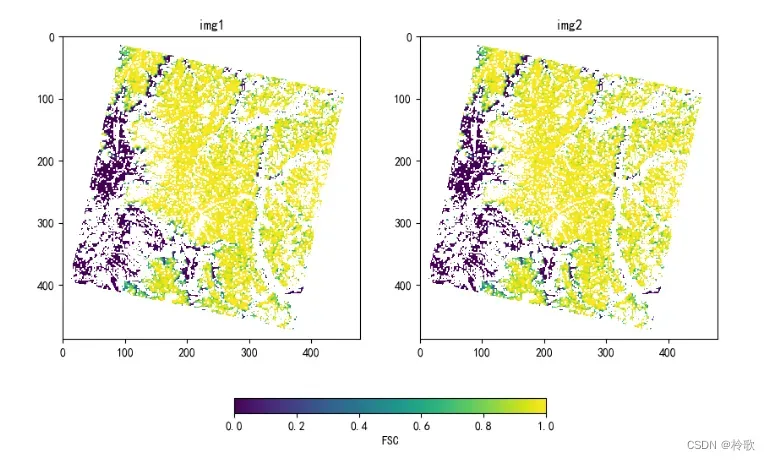
(1)使用 Rioxarray 读取并展示图像:
import rasterio
import rioxarray
import matplotlib.pyplot as plt

plt.rcParams['font.sans-serif'] = ['SimHei']
plt.rcParams['axes.unicode_minus'] = False

img_path = '../images/tiff_img.tif'

img = rioxarray.open_rasterio(img_path)
print(img.shape)  # (22, 488, 480),第一维为通道数
print(type(img))  # <class 'xarray.core.dataarray.DataArray'>
print(type(img.values))  # <class 'numpy.ndarray'>

fig, axes = plt.subplots(1, 2, figsize=(10, 6))
for ax in axes.flat:
    ax_img = ax.imshow(img[0], cmap='viridis')
for ax, title in zip(axes.flat, ['img1', 'img2']):
    ax.set_title(title)
fig.colorbar(mappable=ax_img, label='FSC', orientation='horizontal', ax=axes, fraction=0.04)  # 图例,fraction可调整大小

plt.show()
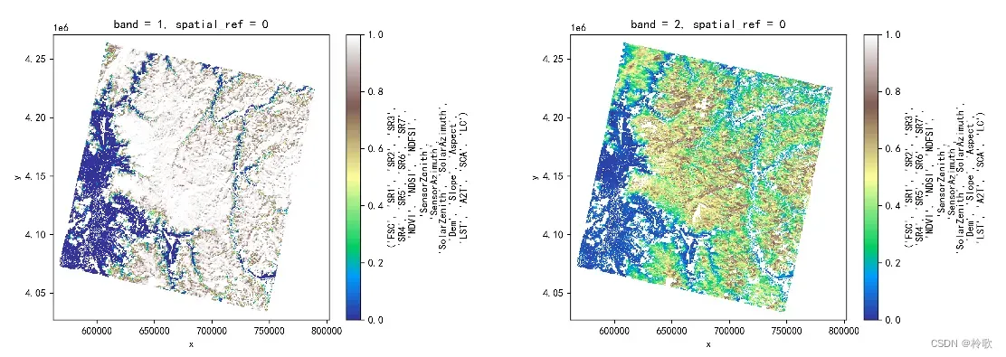
也可以用另一种形式展示(注意如果使用 Rasterio 读取图像则无法使用该方式展示图像):
plt.figure(dpi=300, figsize=(15, 5))
plt.subplots_adjust(hspace=0.2, wspace=0.5)
plt.subplot(1, 2, 1)
img[0].plot(cmap='terrain')  # getting the first band
plt.subplot(1, 2, 2)
img[1].plot(cmap='terrain')
# plt.savefig('1.png', dpi=300, bbox_inches='tight', pad_inches=0)
plt.show()
(2)使用 Rasterio 读取图像:
img = rasterio.open(img_path).read()
print(img.shape)  # (22, 488, 480)
print(type(img))  # <class 'numpy.ndarray'>
(3)转换为 Tensor 类型:
import torch
import numpy as np

img_torch = torch.tensor(np.array(img.values), dtype=torch.float32)  # Rioxarray转Tensor
print(img_torch.shape)  # torch.Size([22, 488, 480])

img_torch = torch.tensor(img, dtype=torch.float32)  # Rasterio转Tensor
print(img_torch.shape)  # torch.Size([22, 488, 480])
(4)将 TIFF 图像逐像素提取出数据构建 CSV 文件:
import os
import tqdm
import pandas as pd
from sklearn.model_selection import train_test_split

def read_image(img_path):
    img = rasterio.open(img_path).read()
    band, height, width = np.shape(img)

    img_data_list = []
    for x in tqdm.trange(height):
        for y in range(width):
            temp = img[::, x, y]
            if np.array(np.isnan(temp), dtype=np.int8).sum() > 0:  # 过滤nan值
                continue
            else:
                img_data_list.append(temp.tolist())

    img_arr = np.array(img_data_list)
    img_arr = np.around(img_arr, 6)  # 将数据四舍五入保留6位小数
    labels = img_arr[:, 0]  # 第一个特征为标签
    dataset = img_arr[:, 1:]  # 之后的特征为训练数据
    print(os.path.basename(img_path), '读取成功!')

    # return dataset, labels
    return img_arr

total_dataset = np.zeros((1, 22), dtype=np.float32)
img_data = read_image(img_path)
total_dataset = np.append(total_dataset, img_data, axis=0)
total_dataset = np.delete(total_dataset, obj=0, axis=0)  # 按行(axis=0)删除第一行(obj=0)元素
print(total_dataset, '\n', np.shape(total_dataset))
# [[0.570768 0.14354  0.159068 ... 0.458602 1.       0.4     ]
#  [0.307365 0.14354  0.159068 ... 0.458602 1.       0.4     ]
#  [0.005285 0.14354  0.159068 ... 0.428406 1.       0.4     ]
#  ...
#  [0.993229 0.393478 0.370807 ... 0.243081 1.       0.8     ]
#  [0.967867 0.370807 0.356894 ... 0.243081 1.       0.8     ]
#  [0.945627 0.321429 0.305714 ... 0.243081 1.       0.8     ]]
#  (116082, 22)

# 一张影像22个波段,每一波段为一种特征,特征名如下,其中FSC既是模型训练时的标签数据也是模型输出数据
feature_name = ['FSC', 'SR1', 'SR2', 'SR3', 'SR4', 'SR5', 'SR6', 'SR7', 'NDVI', 'NDSI',
                'NDFSI', 'SensorZenith', 'SensorAzimuth', 'SolarZenith', 'SolarAzimuth',
                'Dem', 'Slope', 'Aspect', 'LST', 'A2T', 'SC', 'LCT']
df = pd.DataFrame(total_dataset, columns=feature_name)
df.to_csv('../data/MODIS_total_data.csv', index=False)
print(df)
#              FSC       SR1       SR2       SR3  ...       LST       A2T   SC  LCT
# 0       0.570768  0.143540  0.159068  0.165776  ...  0.447205  0.458602  1.0  0.4
# 1       0.307365  0.143540  0.159068  0.165776  ...  0.447205  0.458602  1.0  0.4
# ...          ...       ...       ...       ...  ...       ...       ...  ...  ...
# 116080  0.967867  0.370807  0.356894  0.384162  ...  0.252946  0.243081  1.0  0.8
# 116081  0.945627  0.321429  0.305714  0.327329  ...  0.252946  0.243081  1.0  0.8
# [116082 rows x 22 columns]

train_data, valid_data = train_test_split(df, test_size=0.3, random_state=1)  # 按7:3的比例划分train_data与valid_data
train_data.to_csv('../data/MODIS_train_data.csv', index=False)
valid_data.to_csv('../data/MODIS_valid_data.csv', index=False)
print(train_data)
print(valid_data)
#             FSC       SR1       SR2  ...       A2T        SC  LCT
# 65463  1.000000  0.868261  0.860124  ...  0.306415  0.954102  0.4
# 71636  0.000000  0.074969  0.090683  ...  0.492837  0.021780  0.4
# ...         ...       ...       ...  ...       ...       ...  ...
# 77708  0.836359  0.252298  0.268199  ...  0.400243  1.000000  0.4
# 98539  0.004958  0.048758  0.073168  ...  0.547051  0.000000  0.4
# [81257 rows x 22 columns]
#              FSC       SR1       SR2  ...       A2T        SC  LCT
# 24035   0.907556  0.579814  0.588075  ...  0.332088  1.000000  0.8
# 26625   0.988592  0.708696  0.702981  ...  0.334435  0.999297  0.4
# ...          ...       ...       ...  ...       ...       ...  ...
# 22745   0.000000  0.054348  0.127143  ...  0.494257  0.532436  0.4
# 31068   0.994422  0.562795  0.532174  ...  0.384267  1.000000  0.4
# [34825 rows x 22 columns]
文章出处登录后可见!
已经登录?立即刷新