新手参加比赛,不足之处敬请谅解
题目链接:链接:https://pan.baidu.com/s/1x1U-kobvPjNMm8xnvS9Gdg
提取码:7id3
目录
任务1 数据探索与清洗
任务1.1 数据探索与预处理
任务1.2 特征编码
任务2 产品营销数据可视化分析
任务2.1
任务2.2
任务2.3
任务2.4
任务3 客户流失因素可视化分析
任务3.1
任务3.2
任务3.3
任务3.4
任务1 数据探索与清洗
分别对短期客户产品购买数据“short-customer-data.csv”(简称短期数据)和长期客户资源信息数据的训练集“long-customer-train.csv”(简称长期数据)进行数据探索与清洗。
任务1.1 数据探索与预处理
(1) 探索短期数据各指标数据的缺失值和“user_id”列重复值,删除缺失值、重复值所在行数据。请在报告中给出处理过程及必要结果,完整的结果保存到文件“result1_1.xlsx”中。
1.首先通过info函数查看数据情况
import pandas as pd
data=pd.read_csv("F:\泰迪杯B题\B题:银行客户忠诚度分析赛题数据\B题:银行客户忠诚度分析赛题数据\short-customer-data.csv")
data.info()
<class 'pandas.core.frame.DataFrame'>
RangeIndex: 41176 entries, 0 to 41175
Data columns (total 14 columns):
# Column Non-Null Count Dtype
--- ------ -------------- -----
0 user_id 41176 non-null object
1 age 41176 non-null int64
2 job 40846 non-null object
3 marital 41096 non-null object
4 education 39446 non-null object
5 default 32580 non-null object
6 housing 40186 non-null object
7 loan 40186 non-null object
8 contact 41176 non-null object
9 month 41176 non-null object
10 day_of_week 41176 non-null object
11 duration 41176 non-null int64
12 poutcome 41176 non-null object
13 y 41176 non-null object
dtypes: int64(2), object(12)
memory usage: 4.4+ MB
2.删除缺失值所在行数据
data.dropna(inplace=True)3. 查看“user_id”列重复值
(data["user_id"].value_counts()).head(20)BA2200001 12
BA2200775 7
BA2239485 7
BA2241169 6
BA2200077 2
BA2241172 2
BA2201983 2
BA2240741 2
BA2200107 2
BA2229101 1
BA2220590 1
BA2208766 1
BA2225619 1
BA2204624 1
BA2227831 1
BA2239381 1
BA2224934 1
BA2224984 1
BA2200497 1
BA2203990 1
Name: user_id, dtype: int644.通过drop_duplicates函数删除重复值所在行数据
data.drop_duplicates(subset=['user_id'],inplace=True)5. 写入excel文件
df1=pd.DataFrame(data)
df1.to_excel('F:\\泰迪杯B题\\B题:银行客户忠诚度分析赛题数据\\result1_1.xlsx',sheet_name='sheet1',index=None)long_data=long_data[~long_data["Age"].isin([0,'-',-1])]2.数据处理
long_data["Age"] = long_data["Age"].str.replace("岁","")
long_data["Age"] = long_data["Age"].str.replace("","")long_data["Age"].unique()array(['52', '41', '42', '61', '39', '44', '53', '48', '60', '32', '38',
'51', '56', '28', '57', '45', '46', '40', '30', '59', '33', '35',
'54', '62', '23', '24', '36', '47', '73', '49', '37', '58', '21',
'55', '29', '70', '34', '43', '31', '27', '50', '66', '26', '20',
'64', '63', '71', '22', '25', '73 ', '75', '18', '1', '65', '72',
'69', '33 ', '25 ', '24 ', '76', '47 ', '74', '19', '77', '0',
'68', '49 ', '67', '63 ', '34 ', '50 ', '64 ', '29 ', '81', '27 ',
'83', '79', '78', '23 ', '30 ', '26 ', '45 ', '77 ', '84', '80',
'92', '32 ', '28 ', '31 ', '66 ', '22 ', '62 ', '46 ', '21 ',
'57 ', '82', '88'], dtype=object)3.写入excel文件
df2=pd.DataFrame(long_data)
df2.to_excel('F:\\泰迪杯B题\\B题:银行客户忠诚度分析赛题数据\\result1_2.xlsx',sheet_name='sheet1',index=None)
任务1.2 特征编码
对短期数据中的字符型数据进行特征编码,如将信用违约情况{‘否’,‘是’}编码为{0,1}。请在报告中给出处理思路、过程及必要结果,完整的结果保存到文件“result1_3.xlsx”中。1.观察数据类型data.dtypesuser_id object
age int64
job object
marital object
education object
default object
housing object
loan object
contact object
month object
day_of_week object
duration int64
poutcome object
y object
dtype: object2.分别求各字符型数据值分布
data["job"].value_counts()admin. 8724
blue-collar 5670
technician 5459
services 2855
management 2310
retired 1212
self-employed 1092
entrepreneur 1088
unemployed 738
housemaid 688
student 609
Name: job, dtype: int64data["marital"].value_counts()married 17472
single 9426
divorced 3547
Name: marital, dtype: int64
data["education"].value_counts()undergraduate 10397
postgraduate 8037
high school 7688
junior college 4312
illiterate 11
Name: education, dtype: int64data["housing"].value_counts()yes 16498
no 13947
Name: housing, dtype: int64data["loan"].value_counts()no 25680
yes 4765
Name: loan, dtype: int64data["contact"].value_counts()cellular 20420
telephone 10025
Name: contact, dtype: int64data["month"].value_counts()may 9718
jul 5075
aug 4667
jun 3608
nov 3492
apr 2112
oct 641
sep 493
mar 482
dec 157
Name: month, dtype: int64data["day_of_week"].value_counts()thu 6388
mon 6274
wed 6116
tue 5939
fri 5728
Name: day_of_week, dtype: int64data["poutcome"].value_counts()nonexistent 25796
failure 3458
success 1191
Name: poutcome, dtype: int64data["y"].value_counts()no 26589
yes 3856
Name: y, dtype: int642.将数据分布为{‘否’,‘是’}编码为{0,1}
data["housing"] = data["housing"].str.replace("yes","1")
data["housing"] = data["housing"].str.replace("no","0")
data["loan"] = data["loan"].str.replace("yes","1")
data["loan"] = data["loan"].str.replace("no","0")
data["default"] = data["default"].str.replace("yes","1")
data["default"] = data["default"].str.replace("no","0")
data["y"] = data["y"].str.replace("yes","1")
data["y"] = data["y"].str.replace("no","0")3.使用sklearn中的独热编码对其它非{yes,no}的具体值特征都转换为哑变量,分别赋值“0”和“1”
ps:数据量较多,为了谨慎处理避免出错,对数据多次处理
from sklearn.preprocessing import OneHotEncoder
index=data.values[:,0:2]
index_data=index #获得ID列
job_marital_education=data.values[:,2:5]
enc=OneHotEncoder() #建立模型对象
df1_new=enc.fit_transform(job_marital_education).toarray() #标志转换
df1_index_education=pd.concat((pd.DataFrame(index_data),pd.DataFrame(df1_new)),axis=1) #组合为数据框
df1_index_education.columns=['user_id', 'age',
                             'admin','blue-collar','entrepreneur','housemaid','management','retired','self-employed','services','student',
                 'technician','unemployed','divorced','married','single',
                             'high school','illiterate','junior college','postgraduate','undergraduate']
df1_index_education.head()
contact_month_week=data.values[:,8:11]
enc=OneHotEncoder() #建立模型对象
df2_new=enc.fit_transform(contact_month_week).toarray() #标志转换
df_index_week=pd.concat((pd.DataFrame(df1_index_education),pd.DataFrame(df2_new)),axis=1) #组合为数据框
df_index_week.columns=['user_id', 'age',
'admin','blue-collar','entrepreneur','housemaid','management','retired','self-employed','services','student',
'technician','unemployed','divorced','married','single',
'high school','illiterate','junior college','postgraduate','undergraduate',
'cellular','telephone','apr','aug','dec','jul','jun','mar','may','nov','oct','sep','fri','mon','thu','tue','wed']
df_index_weekdefault_loan=data.values[:,5:8]
df_now=pd.concat((pd.DataFrame(df_index_week),pd.DataFrame(default_loan)),axis=1) #组合为数据框
df_now.columns=['user_id', 'age',
'admin','blue-collar','entrepreneur','housemaid','management','retired','self-employed','services','student',
'technician','unemployed','divorced','married','single',
'high school','illiterate','junior college','postgraduate','undergraduate',
'cellular','telephone','apr','aug','dec','jul','jun','mar','may','nov','oct','sep','fri','mon','thu','tue','wed','default',
'housing','loan']
df_nowdata["y"]=data["y"].astype(dtype='int')
poutcome=data.values[:,11:]
data["y"]=data["y"].astype(dtype='int')
poutcome=data.values[:,12:]
enc=OneHotEncoder() #建立模型对象
df3_new=enc.fit_transform(poutcome).toarray() #标志转换
df_all=pd.concat((pd.DataFrame(df_index_week),pd.DataFrame(df3_new)),axis=1) #组合为数据框
df_all.columns=['user_id', 'age',
'admin','blue-collar','entrepreneur','housemaid','management','retired','self-employed','services','student',
'technician','unemployed','divorced','married','single',
'high school','illiterate','junior college','postgraduate','undergraduate',
'cellular','telephone','apr','aug','dec','jul','jun','mar','may','nov','oct','sep','fri','mon','thu','tue','wed',
'failure','nonexistent','success','1','0']
df_all.drop("0",axis=1,inplace=True)
df_all.drop("1",axis=1,inplace=True)
df_alllast=data.values[:,11:14:2]
data_last=pd.concat((pd.DataFrame(df_all),pd.DataFrame(last)),axis=1) #组合为数据框
data_last.columns=['user_id', 'age',
'admin','blue-collar','entrepreneur','housemaid','management','retired','self-employed','services','student',
'technician','unemployed','divorced','married','single',
'high school','illiterate','junior college','postgraduate','undergraduate',
'cellular','telephone','apr','aug','dec','jul','jun','mar','may','nov','oct','sep','fri','mon','thu','tue','wed','failure','nonexistent','success','duration','y']
data_last这里到后面做任务2的时候才发现漏了几列数据[o(╥﹏╥)o],然后又回来补上
bb=data.values[:,5:8]
data_data=pd.concat((pd.DataFrame(data_last),pd.DataFrame(bb)),axis=1) #组合为数据框
data_data.columns=['user_id', 'age',
                             'admin','blue-collar','entrepreneur','housemaid','management','retired','self-employed','services','student',
                 'technician','unemployed','divorced','married','single',
                             'high school','illiterate','junior college','postgraduate','undergraduate',
                      'cellular','telephone','apr','aug','dec','jul','jun','mar','may','nov','oct','sep','fri','mon','thu','tue','wed',
               'failure','nonexistent','success','duration','y','default','housing','loan']
data_data
3.最后写入Excel
df3=pd.DataFrame(data_data)
df3.to_excel('F:\\泰迪杯B题\\B题:银行客户忠诚度分析赛题数据\\result1_3.xlsx',sheet_name='sheet1',index=None)
任务1完!
任务2 产品营销数据可视化分析
基于短期数据分析不同指标客户与购买银行产品行为的关联性,挖掘短期客户对银行的忠诚度。任务2.1
计算短期数据所有指标之间的相关性,绘制相关系数热力图,并在报告中对结果进行必要分析。import pandas as pd
import matplotlib.pyplot as plt
import seaborn as sns
import missingno as ms
import plotly.express as px
import plotly.graph_objs as go
import plotly.figure_factory as ff
from plotly.subplots import make_subplots
import plotly.offline as pyo
pyo.init_notebook_mode()
sns.set_style('darkgrid')
plt.style.use('fivethirtyeight')
%matplotlib inline
import shap
plt.rc('figure',figsize=(18,9))
short_data=pd.read_excel('F:\\泰迪杯B题\\B题:银行客户忠诚度分析赛题数据\\result1_3.xlsx')corr=short_data.corr() #仅针对数值连续变量
plt.figure(figsize=(20,15))
sns.heatmap(corr
,annot=True
,linewidths=2
,linecolor='lightgrey')
plt.show()
任务2.2
在同一画布中,绘制反映两种产品购买结果下不同年龄客户量占比的分组柱状图,x 轴为年龄,y 轴为占比数值,并在报告中对结果进行必要分析。num_20_1=0
num_30_1=0
num_40_1=0
num_50_1=0
num_60_1=0
num_70_1=0
num_80_1=0
num_90_1=0
num_100_1=0
for i in range(len(short_data["age"])):
if short_data.loc[i,'age']<=20 and short_data.loc[i,'y']==1:
num_20_1+=1
if 21<=short_data.loc[i,'age']<=30 and short_data.loc[i,'y']==1:
num_30_1+=1
if 31<=short_data.loc[i,'age']<=40 and short_data.loc[i,'y']==1:
num_40_1+=1
if 41<=short_data.loc[i,'age']<=50 and short_data.loc[i,'y']==1:
num_50_1+=1
if 51<=short_data.loc[i,'age']<=60 and short_data.loc[i,'y']==1:
num_60_1+=1
if 61<=short_data.loc[i,'age']<=70 and short_data.loc[i,'y']==1:
num_70_1+=1
if 71<=short_data.loc[i,'age']<=80 and short_data.loc[i,'y']==1:
num_80_1+=1
if 81<=short_data.loc[i,'age']<=90 and short_data.loc[i,'y']==1:
num_90_1+=1
if 91<=short_data.loc[i,'age']<=100 and short_data.loc[i,'y']==1:
num_100_1+=1
num_20_0=0
num_30_0=0
num_40_0=0
num_50_0=0
num_60_0=0
num_70_0=0
num_80_0=0
num_90_0=0
num_100_0=0
for i in range(len(short_data["age"])):
if short_data.loc[i,'age']<=20 and short_data.loc[i,'y']==0:
num_20_0+=1
if 21<=short_data.loc[i,'age']<=30 and short_data.loc[i,'y']==0:
num_30_0+=1
if 31<=short_data.loc[i,'age']<=40 and short_data.loc[i,'y']==0:
num_40_0+=1
if 41<=short_data.loc[i,'age']<=50 and short_data.loc[i,'y']==0:
num_50_0+=1
if 51<=short_data.loc[i,'age']<=60 and short_data.loc[i,'y']==0:
num_60_0+=1
if 61<=short_data.loc[i,'age']<=70 and short_data.loc[i,'y']==0:
num_70_0+=1
if 71<=short_data.loc[i,'age']<=80 and short_data.loc[i,'y']==0:
num_80_0+=1
if 81<=short_data.loc[i,'age']<=90 and short_data.loc[i,'y']==0:
num_90_0+=1
if 91<=short_data.loc[i,'age']<=100 and short_data.loc[i,'y']==0:
num_100_0+=1
total_1=num_20_1+num_30_1+num_40_1+num_50_1+num_60_1+num_70_1+num_80_1+num_90_1+num_100_1
total_0=num_20_0+num_30_0+num_40_0+num_50_0+num_60_0+num_70_0+num_80_0+num_90_0+num_100_0
from matplotlib import pyplot as plt
font = {'family': 'MicroSoft YaHei',
'weight': 'bold',
'size': '12'}
matplotlib.rc("font",**font)
x=["<20","21-30","31-40","41-50","51-60","61-70","71-80","81-90","91-100"]
y_1=[num_20_1/total_1,num_30_1/total_1,num_40_1/total_1,num_50_1/total_1,num_60_1/total_1,num_70_1/total_1,num_80_1/total_1,num_90_1/total_1,num_100_1/total_1]
y_0=[num_20_0/total_0,num_30_0/total_0,num_40_0/total_0,num_50_0/total_0,num_60_0/total_0,num_70_0/total_0,num_80_0/total_0,num_90_0/total_0,num_100_0/total_0]
ax=plt.subplot(1,2,1)
plt.bar(x,y_1,color='orange')
plt.xlabel("年龄分组")
plt.xticks(x)
plt.ylabel("人数占比")
plt.title('客户购买结果为1')
ax=plt.subplot(1,2,2)
plt.bar(x,y_0,color='green')
plt.grid(color='#95a5a6',linestyle='--',linewidth=1,axis='y',alpha=0.5)
plt.xlabel("年龄分组")
plt.xticks(x)
plt.ylabel("人数占比")
plt.title('客户购买结果为0')
plt.grid(color='#95a5a6',linestyle='--',linewidth=1,axis='y',alpha=0.5)
plt.show()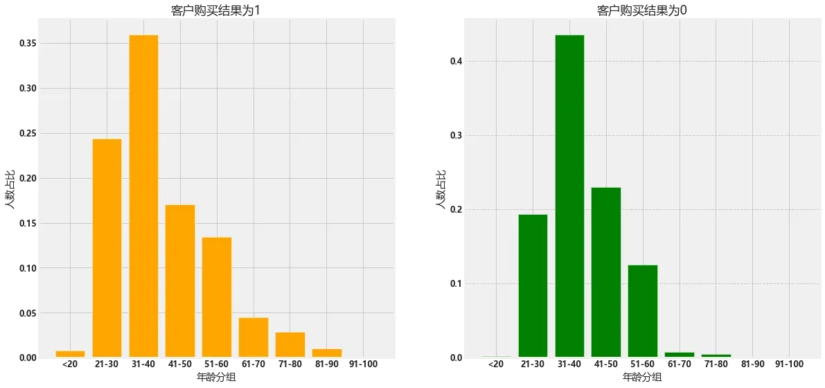
任务2.3
在同一画布中,绘制蓝领(blue-collar)与学生(student)的产品购买情况饼图,并设定饼图的标签,显示产品购买情况的占比。blue_1=0
student_1=0
for i in range(len(short_data["age"])):
if short_data.loc[i,"blue-collar"]==1 and short_data.loc[i,'y']==1:
blue_1+=1
if short_data.loc[i,"student"]==1 and short_data.loc[i,'y']==1:
student_1+=1
blue_0=0
student_0=0
for i in range(len(short_data["age"])):
if short_data.loc[i,"blue-collar"]==1 and short_data.loc[i,'y']==0:
blue_0+=1
if short_data.loc[i,"student"]==1 and short_data.loc[i,'y']==0:
student_0+=1
num1=[blue_1,student_1]
num0=[blue_0,student_0]
colors = ['blue','yellow']
# #设置突出模块偏移值
expodes = (0,0)
#设置绘图属性并绘图
ax=plt.subplot(1,2,1)
plt.pie(num1,explode=expodes,labels=labels,shadow=True,colors=colors)
plt.title("产品购买结果为1")
plt.axis('equal')
ax=plt.subplot(1,2,2)
plt.pie(num0,explode=expodes,labels=labels,shadow=True,colors=colors)
plt.title("产品购买结果为0")
plt.axis('equal')
plt.show()
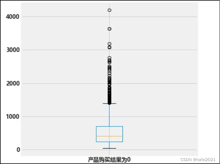
任务2.4
以产品购买结果为 x 轴、拜访客户的通话时长为 y 轴,绘制拜访客户的通话时长箱线图,并在报告中对结果进行必要分析。x=["产品购买结果为1","产品购买结果为0"]
y_1=[]
y_0=[]
for i in range(len(short_data["age"])):
if short_data.loc[i,'y']==0:
y_1.append(short_data.loc[i,'duration'])
if short_data.loc[i,'y']==1:
y_0.append(short_data.loc[i,'duration'])
dt = pd.DataFrame({'产品购买结果为0': y_0})
dt = pd.DataFrame({'产品购买结果为1': y_1})
dt.boxplot() #对数据框中每列画箱线图,pandas自己有处理的过程
plt.show()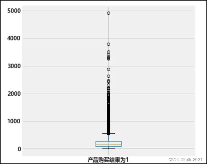
任务3 客户流失因素可视化分析
基于长期数据分析导致银行客户流失的因素,并进行可视化呈现。任务3.1
在同一画布中,绘制反映两种流失情况下不同年龄客户量占比的折线图,x 轴为年龄,y 轴为占比数值import pandas as pd
long_data=pd.read_excel('F:\\泰迪杯B题\\B题:银行客户忠诚度分析赛题数据\\result1_2.xlsx')
num_20_1=0
num_30_1=0
num_40_1=0
num_50_1=0
num_60_1=0
num_70_1=0
num_80_1=0
num_90_1=0
num_100_1=0
for i in range(len(short_data["Age"])):
if short_data.loc[i,'Age']<=20 and short_data.loc[i,'Exited']==1:
num_20_1+=1
if 21<=short_data.loc[i,'Age']<=30 and short_data.loc[i,'Exited']==1:
num_30_1+=1
if 31<=short_data.loc[i,'Age']<=40 and short_data.loc[i,'Exited']==1:
num_40_1+=1
if 41<=short_data.loc[i,'Age']<=50 and short_data.loc[i,'Exited']==1:
num_50_1+=1
if 51<=short_data.loc[i,'Age']<=60 and short_data.loc[i,'Exited']==1:
num_60_1+=1
if 61<=short_data.loc[i,'Age']<=70 and short_data.loc[i,'Exited']==1:
num_70_1+=1
if 71<=short_data.loc[i,'Age']<=80 and short_data.loc[i,'Exited']==1:
num_80_1+=1
if 81<=short_data.loc[i,'Age']<=90 and short_data.loc[i,'Exited']==1:
num_90_1+=1
if 91<=short_data.loc[i,'Age']<=100 and short_data.loc[i,'Exited']==1:
num_100_1+=1
num_20_0=0
num_30_0=0
num_40_0=0
num_50_0=0
num_60_0=0
num_70_0=0
num_80_0=0
num_90_0=0
num_100_0=0
for i in range(len(short_data["Age"])):
if short_data.loc[i,'Age']<=20 and short_data.loc[i,'Exited']==0:
num_20_0+=1
if 21<=short_data.loc[i,'Age']<=30 and short_data.loc[i,'Exited']==0:
num_30_0+=1
if 31<=short_data.loc[i,'Age']<=40 and short_data.loc[i,'Exited']==0:
num_40_0+=1
if 41<=short_data.loc[i,'Age']<=50 and short_data.loc[i,'Exited']==0:
num_50_0+=1
if 51<=short_data.loc[i,'Age']<=60 and short_data.loc[i,'Exited']==0:
num_60_0+=1
if 61<=short_data.loc[i,'Age']<=70 and short_data.loc[i,'Exited']==0:
num_70_0+=1
if 71<=short_data.loc[i,'Age']<=80 and short_data.loc[i,'Exited']==0:
num_80_0+=1
if 81<=short_data.loc[i,'Age']<=90 and short_data.loc[i,'Exited']==0:
num_90_0+=1
if 91<=short_data.loc[i,'Age']<=100 and short_data.loc[i,'Exited']==0:
num_100_0+=1
total_1=num_20_1+num_30_1+num_40_1+num_50_1+num_60_1+num_70_1+num_80_1+num_90_1+num_100_1
total_1
total_0=num_20_0+num_30_0+num_40_0+num_50_0+num_60_0+num_70_0+num_80_0+num_90_0+num_100_0
total_0
import pandas as pd
import matplotlib
from matplotlib import pyplot as plt
font = {'family': 'MicroSoft YaHei',
'weight': 'bold',
'size': '12'}
matplotlib.rc("font",**font)
x=["<20","21-30","31-40","41-50","51-60","61-70","71-80","81-90","91-100"]
y_1=[num_20_1/total_1,num_30_1/total_1,num_40_1/total_1,num_50_1/total_1,num_60_1/total_1,num_70_1/total_1,num_80_1/total_1,num_90_1/total_1,num_100_1/total_1]
y_0=[num_20_0/total_0,num_30_0/total_0,num_40_0/total_0,num_50_0/total_0,num_60_0/total_0,num_70_0/total_0,num_80_0/total_0,num_90_0/total_0,num_100_0/total_0]
plt.figure(figsize=(12,5))
ax=plt.subplot(1,2,1)
plt.plot(x,y_1,color='orange')
plt.xlabel("年龄分组")
plt.xticks(x)
plt.ylabel("人数占比")
plt.title('客户流失')
ax=plt.subplot(1,2,2)
plt.plot(x,y_0,color='green')
plt.grid(color='#95a5a6',linestyle='--',linewidth=1,axis='y',alpha=0.5)
plt.xlabel("年龄分组")
plt.xticks(x)
plt.ylabel("人数占比")
plt.title('客户不流失')
plt.grid(color='#95a5a6',linestyle='--',linewidth=1,axis='y',alpha=0.5)
plt.show()
任务3.2
在同一画布中,绘制反映两种流失情况下客户信用资格与年龄分布的散点图,x 轴为年龄,y 轴为信用资格。x_1=[]
y_1=[]
x_0=[]
y_0=[]
for i in range(len(short_data["Age"])):
if short_data.loc[i,'Exited']==1:
x1=short_data.loc[i,'Age']
y1=short_data.loc[i,'CreditScore']
x_1.append(x1)
y_1.append(y1)
if short_data.loc[i,'Exited']==0:
x0=short_data.loc[i,'Age']
y0=short_data.loc[i,'CreditScore']
x_0.append(x0)
y_0.append(y0)
fig=plt.figure(figsize=(12,5),dpi=100)
ax=plt.subplot(1,2,1)
plt.scatter(x_1,y_1,s=1,)
plt.xlabel("年龄")
plt.ylabel("信用资格")
plt.title('客户流失')
ax=plt.subplot(1,2,2)
plt.scatter(x_0,y_0,s=1,)
plt.xlabel("年龄")
# plt.ylabel("信用资格")
plt.yticks([])
plt.title('客户不流失')
plt.show()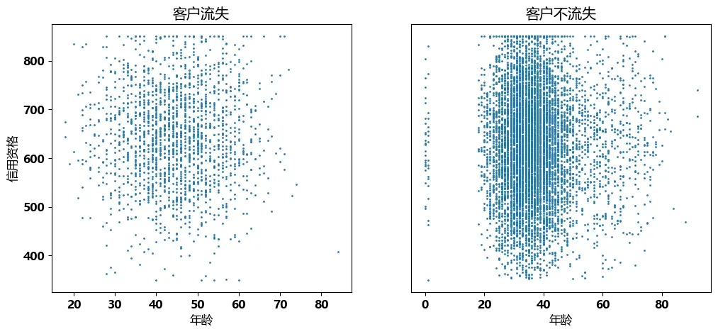
任务3.3
构造包含各账号户龄在不同流失情况下的客户量占比透视表(详见表 4),并在同一画布中绘制反映两种流失情况的客户各账号户龄占比量的堆叠柱状图,x 轴为客户的户龄,y 轴为占比量。
count_0_0=0
count_1_0=0
count_2_0=0
count_3_0=0
count_4_0=0
count_5_0=0
count_6_0=0
count_7_0=0
count_8_0=0
count_9_0=0
count_10_0=0
count_0=[count_0_0,count_1_0,count_2_0,count_3_0,count_4_0,count_5_0,count_6_0,count_7_0,count_8_0,count_9_0,count_10_0]
count_0_1=0
count_1_1=0
count_2_1=0
count_3_1=0
count_4_1=0
count_5_1=0
count_6_1=0
count_7_1=0
count_8_1=0
count_9_1=0
count_10_1=0
count_1=[count_0_1,count_1_1,count_2_1,count_3_1,count_4_1,count_5_1,count_6_1,count_7_1,count_8_1,count_9_1,count_10_1]
for i in range(len(short_data["Age"])):
    if short_data.loc[i,'Exited']==1:
        a1=short_data.loc[i,'Tenure']
        if a1==0:
            count_0_1+=1
        if a1==1:
            count_1_1+=1
        if a1==2:
            count_2_1+=1
        if a1==3:
            count_3_1+=1
        if a1==4:
            count_4_1+=1
        if a1==5:
            count_5_1+=1
        if a1==6:
            count_6_1+=1
        if a1==7:
            count_7_1+=1
        if a1==8:
            count_8_1+=1
        if a1==9:
            count_9_1+=1
        if a1==10:
            count_10_1+=1
    if short_data.loc[i,'Exited']==0:
        a2=short_data.loc[i,'Tenure']
        if a2==0:
            count_0_0+=1
        if a2==1:
            count_1_0+=1
        if a2==2:
            count_2_0+=1
        if a2==3:
            count_3_0+=1
        if a2==4:
            count_4_0+=1
        if a2==5:
            count_5_0+=1
        if a2==6:
            count_6_0+=1
        if a2==7:
            count_7_0+=1
        if a2==8:
            count_8_0+=1
        if a2==9:
            count_9_0+=1
        if a2==10:
            count_10_0+=1
得到透视表:
total_0=0
total_1=0
for i in range(0,11):
    total_0+=count_0[i]
    total_1+=count_1[i]
total_0
total_1
for i in range(0,11):
    count_0[i]=count_0[i]/total_0
    count_1[i]=count_1[i]/total_1
data_1={'count_0':count_0,'count_1':count_1}
df_1=pd.DataFrame(data_1)
df_1.plot(kind='bar',stacked=True,alpha=0.5) 
任务3.4
按照表 5 和表 6 对账号户龄和客户金融资产进行划分,并分别进行特征编码作为新的客户特征,其中客户状态存于“Status”列,资产阶段存于“AssetStage”列,编码结果保存到文件“result3.xlsx”中。
Status=[]
AssetStage=[]

for i in range(len(short_data["Age"])):
    if 0<=short_data.loc[i,'Tenure']<=3:
        Status[i]="新客户"
    if 3<short_data.loc[i,'Tenure']<=6:
        Status[i]="稳定客户"
    if short_data.loc[i,'Tenure']>6:
        Status[i]="老客户"
for i in range(len(short_data["Age"])):
    if 0<=short_data.loc[i,'Balance']<=50000:
        AssetStage[i]="低资产"
    if 50000<short_data.loc[i,'Balance']<=90000:
        AssetStage[i]="中下资产"
    if 90000<short_data.loc[i,'Balance']<=120000:
        AssetStage[i]="中上资产"
    if short_data.loc[i,'Balance']>120000:
        AssetStage[i]="高资产"
data_1={'Status':Status,'AssetStage':AssetStage}
df_1=pd.DataFrame(data_1)
df_1.to_excel('F:\\泰迪杯B题\\B题:银行客户忠诚度分析赛题数据\\result3.xlsx',sheet_name='sheet1',index=None)test=pd.read_excel('F:\\泰迪杯B题\\B题:银行客户忠诚度分析赛题数据\\任务3.4.2.xlsx')
new_lower=0
new_low=0
new_high=0
new_higher=0
old_lower=0
old_low=0
old_high=0
old_higher=0
for i in range(len(test['Exited'])):
if test.loc[i,'Exited']==1 and test.loc[i,'Status']=='新客户'and test.loc[i,'AssetStage']=="低资产":
new_lower+=1
if test.loc[i,'Exited']==1 and test.loc[i,'Status']=='新客户'and test.loc[i,'AssetStage']=="中下资产":
new_low+=1
if test.loc[i,'Exited']==1 and test.loc[i,'Status']=='新客户'and test.loc[i,'AssetStage']=="中上资产":
new_high+=1
if test.loc[i,'Exited']==1 and test.loc[i,'Status']=='新客户'and test.loc[i,'AssetStage']=="高资产":
new_higher+=1
if test.loc[i,'Exited']==0 and test.loc[i,'Status']=='老客户'and test.loc[i,'AssetStage']=="低资产":
old_lower+=1
if test.loc[i,'Exited']==0 and test.loc[i,'Status']=='老客户'and test.loc[i,'AssetStage']=="中下资产":
old_low+=1
if test.loc[i,'Exited']==0 and test.loc[i,'Status']=='老客户'and test.loc[i,'AssetStage']=="中上资产":
old_high+=1
if test.loc[i,'Exited']==0 and test.loc[i,'Status']=='老客户'and test.loc[i,'AssetStage']=="高资产":
old_higher+=1
new=[new_lower,new_low,new_high,new_higher]
old=[old_lower,old_low,old_high,old_higher]
data_2={'new_lower':[180],'new_low':[57],'new_high':[181],'new_higher':[246],
'old_lower':[1066],'old_low':[234],'old_high':[536],'old_higher':[800]}
df_2=pd.DataFrame(data_2)
plt.figure(figsize=(10,5))
sns.heatmap(df_2,vmax=1300,vmin=100)
ps:由于篇幅太长,暂时先写到这吧。剩下的会写在另一篇,再做个比赛总结
2022第五届“泰迪杯”数据分析技能赛-B题-银行客户忠诚度分析(下)链接:https://blog.csdn.net/weixin_60200880/article/details/127939604?spm=1001.2014.3001.5502
文章出处登录后可见!