目录
一 、tkinter库的Canvas图形绘制方法
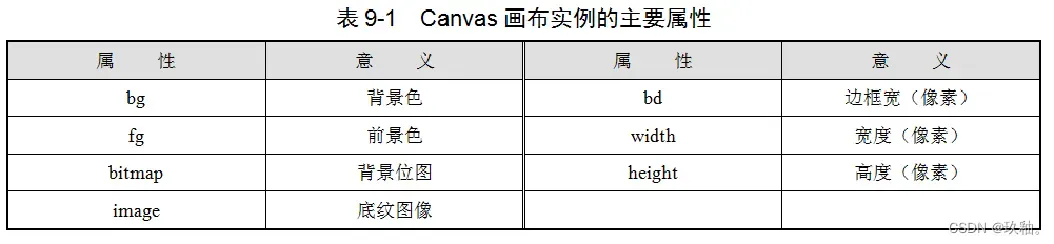
1.创建画布和颜色填充
Canvas画布的坐标原点在左上角,默认单位是像素,x轴向右为正,y轴向下为正。
在320×240的窗体上创建高200,宽280的画布,并填充红色。
from tkinter import *
root=Tk()
root.geometry('320x240')
mycanvas=Canvas(root,bg='red',height=200,width=280)
mycanvas.pack()
btn1=Button(root,text='关闭',command=root.destroy)
btn1.pack()
root.mainloop()
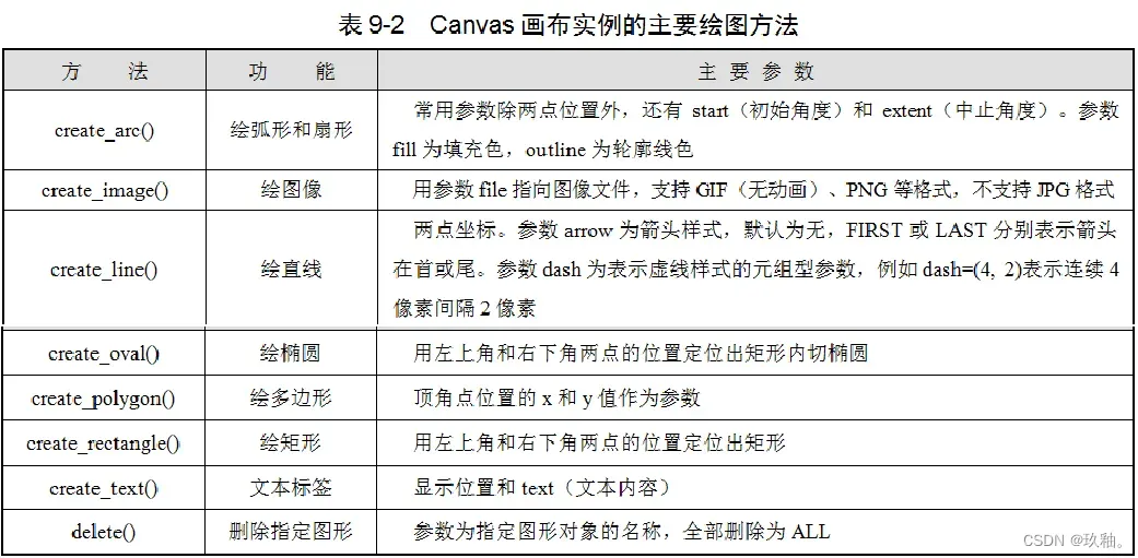
2.绘制图形
在320×240的窗体上创建高200像素,宽300像素的画布,鼠标单击画布,依次绘出:从(90,10)到(200,200)点的矩形;从(90,10)到(200,200)点的内切椭圆并填充绿色;从(90,10)到(200,200)点的内切扇形并填充粉红色;连接(20,180)、(150,10)和(290,180)三点形成蓝色框线且无色填充的三角形;从(10,105)到(290,105)点的红色直线;以(50,10)为起点用RGB”#123456″颜色绘制文本标签“我的画布”。单击“清空”按钮删除所有图形。
from tkinter import *
root=Tk()
root.geometry('320x240')
def draw(event):
    # 画矩形
    mycanvas.create_rectangle(90,10,200,200)
    # 画椭圆,填充绿色
    mycanvas.create_oval(90,10,200,200,fill='green')
    # 画扇形
    mycanvas.create_arc(90,10,200,200,fill='pink')
    # 画多边形(三角形),前景色为蓝色,无填充色
    mycanvas.create_polygon(20,180,150,10,290,180,
                                 outline='blue',fill='')
    # 画直线
    mycanvas.create_line(10,105,290,105,fill='red')
    # 写文字,颜色为十六进制RGB字符串
    mycanvas.create_text(50,10,text='我的画布',fill='#123456')
def delt():
    # 删除画布上的所有图形
    mycanvas.delete(ALL)

mycanvas=Canvas(root,width=300,height=200)
mycanvas.pack()
mycanvas.bind('< Button- 1>',draw)   # 画布绑定鼠标单击事件
btnclear=Button(root,text='清空',command=delt)
btnclear.pack()
root.mainloop()
3.呈现位图图像
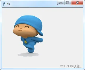
Canvas画布支持呈现位图图像文件,文件类型包括GIF(无动画)、PNG等格式,但不支持JPG格式。 【例9-3】 在320×240的窗体上创建画布,并呈现C:\1.gif图像。
from tkinter import *
root=Tk()
root.geometry('320x240')
mycanvas=Canvas(root)
mycanvas.pack()
photo=PhotoImage(file='c:/1.gif')
mycanvas.create_image(100,100,image=photo)
root.mainloop()
4.利用鼠标事件绘图
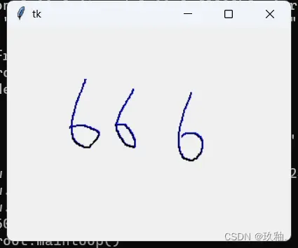
利用按住鼠标左键移动的鼠标事件,不断读取鼠标当前位置,每次扩张1个像素绘制椭圆点,即可在画布上留下鼠标轨迹。 【例9-4】 在320×240的窗体上创建画布,并以蓝色笔创建鼠标画板。
from tkinter import *
root = Tk()
def move(event):
    x=event.x
    y=event.y
    w.create_oval(x,y,x+1,y+1,fill='blue')

w = Canvas(root, width=320, height=240)
w.pack()
w.bind('<B1-Motion>',move)
root.mainloop()
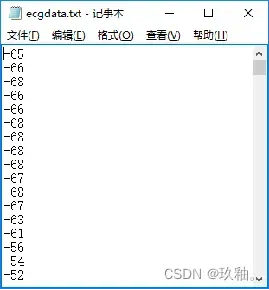
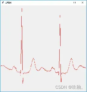
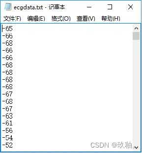
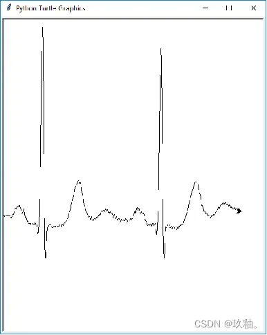
5. 读取
读取“ecgdata.txt”的心电图数据,绘制心电图
import tkinter
root=tkinter.Tk()
root.title('心电图')
cv=tkinter.Canvas(root, width=500, height=500)
cv.pack()
ecg=list(open('ecgdata.txt','r'))
x=0
while x<len(ecg)-1:
    #y轴正方向向下。去掉换行符转换为整数,再向下移动300
    y=-int(ecg[x][:-1])+300
    y1=-int(ecg[x+1][:-1])+300
    cv.create_line(x,y,x+1,y1,fill='red')
    x+=1
root.mainloop()
6.Canvas画布上的函数图形绘制
用create_line()方法可在画布上绘制直线,而随着变量的变化,用该方法连续绘制微直线,即可得到函数的图形。
“分而治之”的计算思维原则。
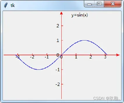
例如:在窗体上创建320×240的画布,以画布中心为原点,用红色绘制带箭头的x和y坐标轴,用蓝色笔绘制正弦曲线y=sinx的函数图形。其中,x、y轴的放大倍数均为40倍,即:x=40t。t以0.01的步长在-~范围内变化取值。
from tkinter import *
import math
root = Tk()
w = Canvas(root, width=320, height=240)
w.pack()
w0=160      # 半宽
h0=120      # 半高
# 画红色的坐标轴线
w.create_line(0, 120, 320, 120, fill="red", arrow=LAST)
w.create_line(160, 240, 160, 0, fill="red", arrow=LAST)
# 标题文字
w.create_text(w0+50,10,text='y=sin(x)')
# x轴刻度
for i in range(-3,4):
    j=i*40
    w.create_line(j+w0, h0, j+w0, h0-5, fill="red")
    w.create_text(j+w0,h0+5,text=str(i))
# y轴刻度
for i in range(-2,3):
    j=i*40
    w.create_line(w0, j+h0, w0+5, j+h0, fill="red")
    w.create_text(w0-10,j+h0,text=str(-i))
# 计算x
def x(t):
    x = t*40   	#  x轴放大40倍
    x+=w0    		# 平移x轴
    return x
# 计算y
def y(t):
    y = math.sin(t)*40    	# y轴放大40倍
    y-=h0              		# 平移y轴
    y = -y              		# y轴值反向
    return y
# 连续绘制微直线
t = -math.pi
while(t<math.pi):
    w.create_line(x(t), y(t), x(t+0.01), y(t+0.01),fill="blue")
    t+=0.01
root.mainloop()
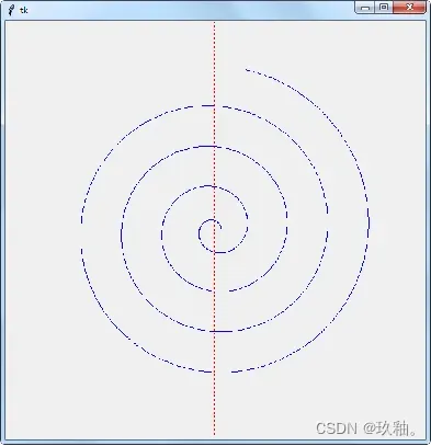
例如:设置坐标原点(x0, y0)为画布的中心(x0, y0分别为画布宽、高的一半),以红色虚线绘制坐标轴,并按以下公式绘制函数曲线: x=(w0 /32)×(cost-tsint) y=(h0 /32)×(sint+tcost) 式中,w0是画布宽的一半,h0是画布高的一半。t的取值范围为0~25,步长为0.01。
from tkinter import *
import math
root = Tk()
w = Canvas(root, width=600, height=600)
w.pack()
# 画红色的坐标轴线(虚线)
w.create_line(0, 300, 600, 300, fill="red", dash=(4, 4))
w.create_line(300, 0, 300, 600, fill="red", dash=(4, 4))
w0=300
h0=300
def x(t):
    x = (w0 / 32) * (math.cos(t) - t*math.sin(t))
    x+=w0    #平移x轴
    return x
def y(t):
    y = (h0 / 32) * (math.sin(t) +t* math.cos(t))
    y-=h0    #平移y轴
    y = -y    #y轴值反向
    return y
t = 0.0
while(t<25):
    w.create_line(x(t), y(t), x(t+0.01), y(t+0.01),fill="blue")
    t+=0.01
root.mainloop()
二、 turtle库的图形绘制方法
turtle也是内置库Python图形绘制库,其绘制方法更为简单,原理如同控制一只“小龟”以不同的方向和速度进行位移而得到其运动轨迹
1、turtle绘图的基本方法
1.坐标位置和方向 setup()方法用于初始化画布窗口大小和位置,参数包括画布窗口宽、画布窗口高、窗口在屏幕的水平起始位置和窗口在屏幕的垂直起始位置
用turtle创建的画布与Canvas不同,其原点(0,0)在画布的中心,坐标方向与数学定义一致,向右、向上为正。
2.画笔 方法color()用于设置或返回画笔颜色
方法pensize()或width()用于设置笔触粗细
3.画笔控制和运动 方法penup()、pu()或up()为抬笔,当笔触移动时不留墨迹;方法pendown(),pd()或down()为落笔,当笔触移动时会留下墨迹。
画笔的移动方法有:向箭头所指方向前进forward()、fd();逆箭头所指方向后退backward(),bk()或back()。
画笔的原地转角方法有:箭头方向左转left()或lt();箭头方向右转right()或rt()。
位移至某点的方法:goto(),setpos()或setposition();画圆的方法:circle();返回原点的方法:home()。 位移速度方法speed(),其取值范围从慢到快为1~10。注意:取0为最快(无移动过程,直接显示目标结果)。 绘图完毕通常用方法done()结束进程。
4.文字 输出文字标签用write()方法,默认参数为输出文本,可选参数有:对齐方式align(left,center,right),font元组型字体设置(字体、字号、字形)。
2、介绍
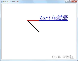
从原点出发至坐标点(-100,100),改为红色,沿光标指向(默认方向为水平向右)前进200像素,改为蓝色,后退100像素,以动画模式输出文字(黑体,36磅,斜体)
from turtle import *
setup(640,480,300,300)
reset()
pensize(5)
goto(-100,100)
color('red')
fd(200)
color('blue')
bk(100)
write('turtle绘图',move=True,font=('黑体',36,'italic'))
done()
3、简单形状图形
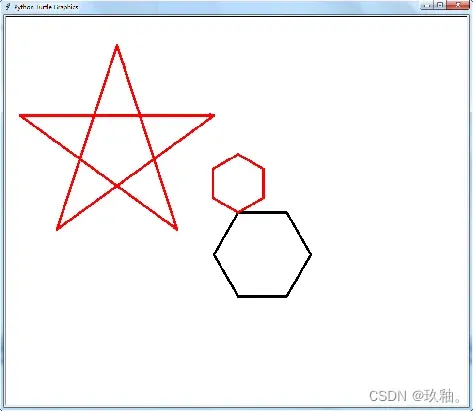
用循环结构可自动重复绘制步骤得出规则图形。 以5像素笔触重复执行“前进100像素,右转60度”的操作共6次,绘制红色正六边形;再用circle()方法画半径为60像素的红色圆内接正六边形;然后抬笔移动至(-50,200)点落笔,重复执行“右转144度,前进400像素”的操作共5次,绘制五角星。
from turtle import *
reset()
pensize(5)
#画正六边形,每步右转60度
for i in range(6):
    fd(100)
    right(60)
#用circle方法画正六边形(半径为60的圆内接正六边形)
color('red')
circle(60,steps=6)
#抬笔移动位置
up()
goto(-50,200)
down()
#画五角星,每步右转144度
for i in range(5):
    right(144)
    fd(400)
done()
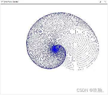
螺纹形状绘制
import turtle as tt
tt.speed(50)
tt.pencolor('blue')
for i in range(100):
    tt.circle(2*i)
    tt.right(4.5)
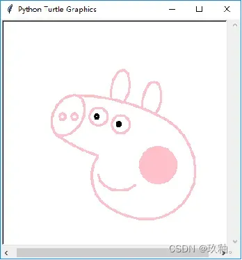
绘制小猪佩奇
import turtle
t = turtle.Turtle()
t.pensize(4) #设置画笔粗
t.color("pink")
turtle.setup(400,400) #设置主窗口的大小
t.speed(20) #设置画笔速度
#画鼻子
t.pu() #提笔
t.goto(-100,0) #画笔移至坐标(-100,100)
t.pd() # 落笔
t.seth(-30) #沿角度-30°
lengh=0.4
for i in range(120):
   if 0<=i<30 or 60<=i<90:
       lengh=lengh+0.08
       t.lt(3) #向左转3度
       t.fd(lengh) #向前移动lengh
   else:
       lengh=lengh-0.08
       t.lt(3)
       t.fd(lengh)
t.pu() # 提笔
t.seth(90) #沿角度90度
t.fd(25) # 向前移动25
t.seth(0) #沿角度0
t.fd(10)
t.pd()
t.pencolor("pink")
t.seth(10)
t.circle(5) # 画一个半径为5的圆
t.pu()
t.seth(0)
t.fd(20)
t.pd()
t.pencolor("pink")
t.seth(10)
t.circle(5)
#画头
t.color("pink")
t.pu()
t.seth(90)
t.fd(41)
t.seth(0)
t.pd()
t.seth(180)
t.circle(300,-30) #画一个半径为300,圆心角为-30°的弧
t.circle(100,-60)
t.circle(80,-100)
t.circle(150,-20)
t.circle(60,-95)
t.seth(161)
t.circle(-300,15)
t.pu()
t.goto(-80,70)
#画耳朵
t.color("pink")
t.pu()
t.seth(90)
t.fd(-7)
t.seth(0)
t.fd(70)
t.pd()
t.seth(100)
t.circle(-50,50)
t.circle(-10,120)
t.circle(-50,54)
t.pu()
t.seth(90)
t.fd(-12)
t.seth(0)
t.fd(30)
t.pd()
t.seth(100)
t.circle(-50,50)
t.circle(-10,120)
t.circle(-50,56)
#画眼睛
t.color("pink")
t.pu()
t.seth(90)
t.fd(-20)
t.seth(0)
t.fd(-95)
t.pd()
t.circle(15)
t.color("black")
t.pu()
t.seth(90)
t.fd(12)
t.seth(0)
t.fd(-3)
t.pd()
t.circle(3)
t.color("pink")
t.pu()
t.seth(90)
t.fd(-25)
t.seth(0)
t.fd(40)
t.pd()
t.circle(15)
t.color("black")
t.pu()
t.seth(90)
t.fd(12)
t.seth(0)
t.fd(-3)
t.pd()
t.begin_fill()
t.circle(3)
t.end_fill()
#画腮红
t.color("pink")
t.pu()
t.seth(90)
t.fd(-95)
t.seth(0)
t.fd(65)
t.pd()
t.begin_fill()
t.circle(30)
t.end_fill()
#画嘴
t.color("pink")
t.pu()
t.seth(90)
t.fd(15)
t.seth(0)
t.fd(-100)
t.pd()
t.ht()  #不显示箭头
t.seth(-80)
t.circle(30,40)
t.circle(40,80)
4、函数图形
用turtle库也可以完成较为复杂的函数二维图形。其方法是:抬笔至图形起点,根据起点、终点、步长及画布的半宽、半高,利用循环逐点计算(x,y)的坐标并移动笔触至该点,最终得到函数图形。 【例9-12】 创建800×800的turtle画布,以画布中心为原点画出坐标轴,并按以下公式绘制函数曲线: x=(w0/4)×(-2sint+sin2t) y=(h0/4)×(2cost-cos2t) 式中,w0是画布宽的一半,h0是画布高的一半。t的取值范围为0~2,步长为0.01。
import math
import turtle
# 自定义从 (x1, y1) 到 (x2, y2)的画直线函数
def drawLine (ttl, x1, y1, x2, y2):
    ttl.penup()
    ttl.goto (x1, y1)
    ttl.pendown()
    ttl.goto (x2, y2)
    ttl.penup()
#逐点计算函数坐标,并按此移动
def drawFunc (ttl, begin, end, step, w0, h0):
    t=begin
    while t < end:
        if t>begin:
            ttl.pendown()
        x = (w0/4)*(-2*math.sin(t)+math.sin(2*t))
        y = (h0/4)*(2*math.cos(t)-math.cos(2*t))
        ttl.goto (x, y)
        t +=  step
    ttl.penup()
def main():
    # 设置画布窗口大小
    turtle.setup (800, 800, 0, 0)
    # 创建turtle对象
    ttl = turtle.Turtle()
    # 画坐标轴
    drawLine (ttl, -400, 0, 400, 0)
    drawLine (ttl, 0, 400, 0, -400)
    # 画函数曲线
    ttl.pencolor ('red')
    ttl.pensize(5)
    drawFunc (ttl, 0, 2*math.pi, 0.01,400,400)
    #对象,起点,终点,步长,半宽,半高
    # 绘图完毕
    turtle.done()
if __name__ == "__main__":
    main()
读取“ecgdata.txt”的心电图数据,绘制心电图。
import turtle
turtle.setup(500,600) #设置主窗口的大小
turtle.speed(20) #设置画笔速度
turtle.pu() #提笔
x=-300
turtle.goto(x,0) #画笔移至坐标
turtle.pd() # 落笔
ecg=list(open('ecgdata.txt','r'))
t=0
while t<len(ecg)-1:
    turtle.goto(t-300,int(ecg[t]))
    t+=1
三、 matplotlib库的图形绘制方法
matplotlib库是用于科学计算数据可视化的常见Python第三方模块。它借鉴了许多Matlab中的函数,可以轻松绘制高质量的线条图、直方图、饼图、散点图及误差线图等二维图形,也可以绘制三维图像,还可以方便地设定图形线条的类型、颜色、粗细及字体的大小等属性。
1、环境安装和基本方法
使用matplotlib库绘图,需要先安装导入numpy科学计算模块库。
如果不想经历烦琐的下载安装过程,也可使用Anaconda等集成安装方式来搭建科学计算环境。
通常,二维图形的绘制是导入matplotlib的pyplot子库所包含的plot函数来完成的。
首先,用导入pyplot子库语句:
import matplotlib.pyplot as plt 然后用 plt.figure(figsize=(w, h),dpi=x) 创建一个绘图对象,并设置对象的宽度比例w和高度比例h。
例如: plt.figure(figsize=(4,3), dpi=200) 为创建一个4:3的每英寸200点分辨率的绘图对象,调用plt.plot()方法在绘图对象中进行绘图。 pyplot()方法也可通过调用subplot()方法增加子图。subplot()方法通常包含三个参数:共有几行、几列、本子图是第几个子图。例如,p1 = plt.subplot(211)或p1 = plt.subplot(2,1,1)表示创建一个2行1列的子图,p1为第一个子图。
plot()方法的参数通常包括x、y轴两个变量及图形的颜色、线型、数据点标记等。
常见的颜色字符有:’r’(红色,red)、’g’(绿色,green)、’b’(蓝色,blue)、’c’(青色,cyan)、’m’(品红,magenta)、’y’(黄色,yellow)、’k’(黑色,black)、’w’(白色,white)等。
常见的线型字符有:’-‘(直线)、’–‘(虚线)、’:’(点线)、’-.’(点画线)等。
常用的描点标记有:’.’(点)、’o’(圆圈)、’s’(方块)、’^’(三角形)、’x’(叉)、’*’(五角星)、’+’(加号)等。
例如: plt.plot(x, y, ‘–*r’)
表示以x和y两个变量绘制红色(r)虚线(–),以星号(*)作为描点标记。
在同一绘图对象中可用plot()方法同时绘制多个图形,例如: plt.plot(x, w, ‘b’,x, y, ‘–*r’, x, z, ‘-.+g’) 表示在同一绘图对象中同时呈现x-w、x-y和x-z三组变量的图形,并且分别以蓝色实线无描点、红色虚线星描点、绿色点画线加号描点表示。
matplotlib默认设置中没有对中文的支持,如果需要使用中文文本标注,应在matplotlib的字体管理器font_manager中专门设置。
例如,将个性化字体对象myfont设为华文宋体:
myfont = matplotlib.font_manager.FontProperties (fname = ‘C:/Windows/Fonts/STSONG.TTF’)
并在输出文字时,使用该字体属性参数:fontproperties=myfont。 由于字体的变化,有时输出负号会受影响(显示不出负号,本例并不涉及),可预设matplotlib.rcParams[‘axes.unicode_minus’] = False解决
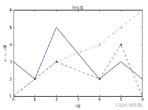
2、在同一绘图对象中,利用不同颜色和标注绘制折线图形
import numpy as np
import matplotlib
import matplotlib.pyplot as plt
myfont = matplotlib.font_manager.FontProperties(fname='C:/Windows/Fonts/STSONG.TTF')
matplotlib.rcParams['axes.unicode_minus'] = False
x = [0, 1, 2, 4, 5, 6]
w = [3, 2, 5, 2, 3, 2]
y = [1, 2, 3, 2, 4, 1]
z = [1, 2, 3, 4, 5, 6]
plt.plot(x, w, 'b',x, y, '--*r', x, z, '-.+g')
plt.xlabel("x轴",fontproperties=myfont)
plt.ylabel("w、y、z轴",fontproperties=myfont)
plt.title("折线图",fontsize=20,fontproperties=myfont)
plt.show()
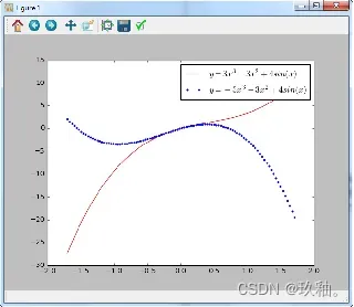
3、二维函数图形绘制
二维函数图形的绘制可调用numpy.linspace()方法,先生成数据系列,再用plot()方法绘图。通式为: numpy.linspace(start, stop, num=50, endpoint=True, retstep=False) 其中,参数依次为自变量起点、终点、生成数据点数、是否包括终点、是否返回间隔。 在同一绘图对象中,分别以红色实线和蓝色点状线绘出x在-1.7~1.7之间变化时的函数图形(100个采样点),并标注其图例和对应公式: y=3×3−3×2+4sin(x) y=−3×3−3×2+4sin(x)。
import numpy as np
import matplotlib.pyplot as plt
x = np.linspace(-1.7, 1.7, 100)
plt.plot(x, 3*x**3-3*x**2+4*np.sin(x),"r",label="$y=3x^{3}-3x^{2}+4sin(x)$")
plt.plot(x, -3*x**3-3*x**2+4*np.sin(x),"b.",label="$y=-3x^{3}-3x^{2}+4sin(x)$")
plt.legend()
plt.show()
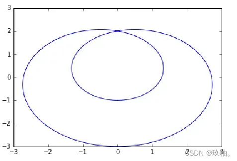
4、按以下公式绘制函数图形
: x=−2sin2t+sint y=−2cos2t+cost 其中,t的取值范围为0~2p,步长为0.02。
import numpy as np
import matplotlib.pyplot as plt
t=np.arange(0,2*np.pi,0.02)
plt.plot(-2*np.sin(2*t)+np.sin(t),-2*np.cos(2*t)+np.cos(t))
plt.show()
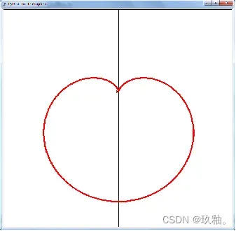
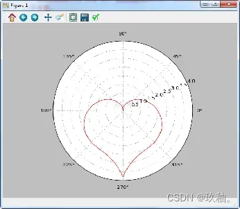
5、用极坐标方式呈现如下公式的红色心状图形:
import numpy as np
import matplotlib.pyplot as plt
t=np.arange(0,2*np.pi,0.02)
plt.subplot(111,polar=True)
w=np.sin(t)*(np.abs(np.cos(t)))**(1/2)/(np.sin(t)+7/5)-2*np.sin(t)+2
plt.plot(t,w,'r')
plt.show()
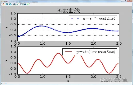
6、创建9:6的200dpi绘图对象
并且在上、下两个子图中分别用蓝色点状线和红色实线呈现x在0.5~2.5范围内变化的函数图形,分别标注坐标轴标签、图例和相应的公式。

![]()
#coding=gbk
import numpy as np
import matplotlib.pyplot as plt
from pylab import *
myfont = matplotlib.font_manager.FontProperties(fname='C:/Windows/Fonts/STSONG.TTF')
matplotlib.rcParams['axes.unicode_minus'] = False

def f1(x):
    return np.exp(-x)*np.cos(2*np.pi*x)

def f2(x):
    return np.sin(2*np.pi*x)*np.cos(3*np.pi*x)

x = np.arange(0.5,2.5,0.02)

plt.figure(figsize=(9,6),dpi=200)
p1 = plt.subplot(211)
p2 = plt.subplot(212)

p1.plot(x,f1(x),"b.",label="$y=e^{-x} \cdot \cos (2 \pi x)$")
p2.plot(x,f2(x),"r-",label="$y=\sin (2 \pi x) \cos (3 \pi x)$",linewidth=2)

p1.axis([0.5,2.5,-1.0,1.5])

p1.set_ylabel("y",fontsize=12)
#p1.set_title('Example Figures',fontsize=20)
p1.set_title('函数曲线',fontsize=20,fontproperties=myfont)
p1.grid(True)
p1.legend()

p2.axis([0.5,2.5,-1.0,1.5])
p2.set_ylabel("y",fontsize=12)
p2.set_xlabel("x",fontsize=12)
p2.legend()

plt.show()
文章出处登录后可见!