🍺相关文章汇总如下🍺:
- 🎈ANSYS二次开发:APDL开发入门准备🎈
- 🎈ANSYS二次开发:后处理使用APDL命令流解析结果文件🎈
- 🎈ANSYS二次开发:Python解析ANSYS结果文件(PyAnsys库)🎈
- 🎈ANSYS二次开发:Python和ANSYS进行交互操作(PyAnsys库,PyDPF)🎈
- 🎈ANSYS二次开发:Python解析ANSYS FLUENT结果文件🎈
文章目录
- 1、下载PyAnsys库
- 2、安装PyAnsys
- 3、官网入门示例
- 4、官网进阶示例
- 4.1 Custom Scalar Visualization(自定义标量可视化)
- 4.2 Cylindrical Nodal Stress(圆柱节点应力)
- 4.3 Shaft Modal Analysis(可视化轴模态分析)
- 4.4 Thermal Analysis(热分析)
- 4.5 Shell Static Analysis(壳静态分析)
- 4.6 Understanding Nodal Diameters from a Cyclic Model Analysis
- 4.7 Stress and Strain from a Cyclic Modal Analysis(循环模态分析中的应力和应变)
- 4.8 Cyclic Model Visualization(动画完整的循环模型)
- 5、个人测试示例
- 结语
1、下载PyAnsys库
1.1 PyAnsys Project(legacy)
https://pypi.org/project/pyansys/
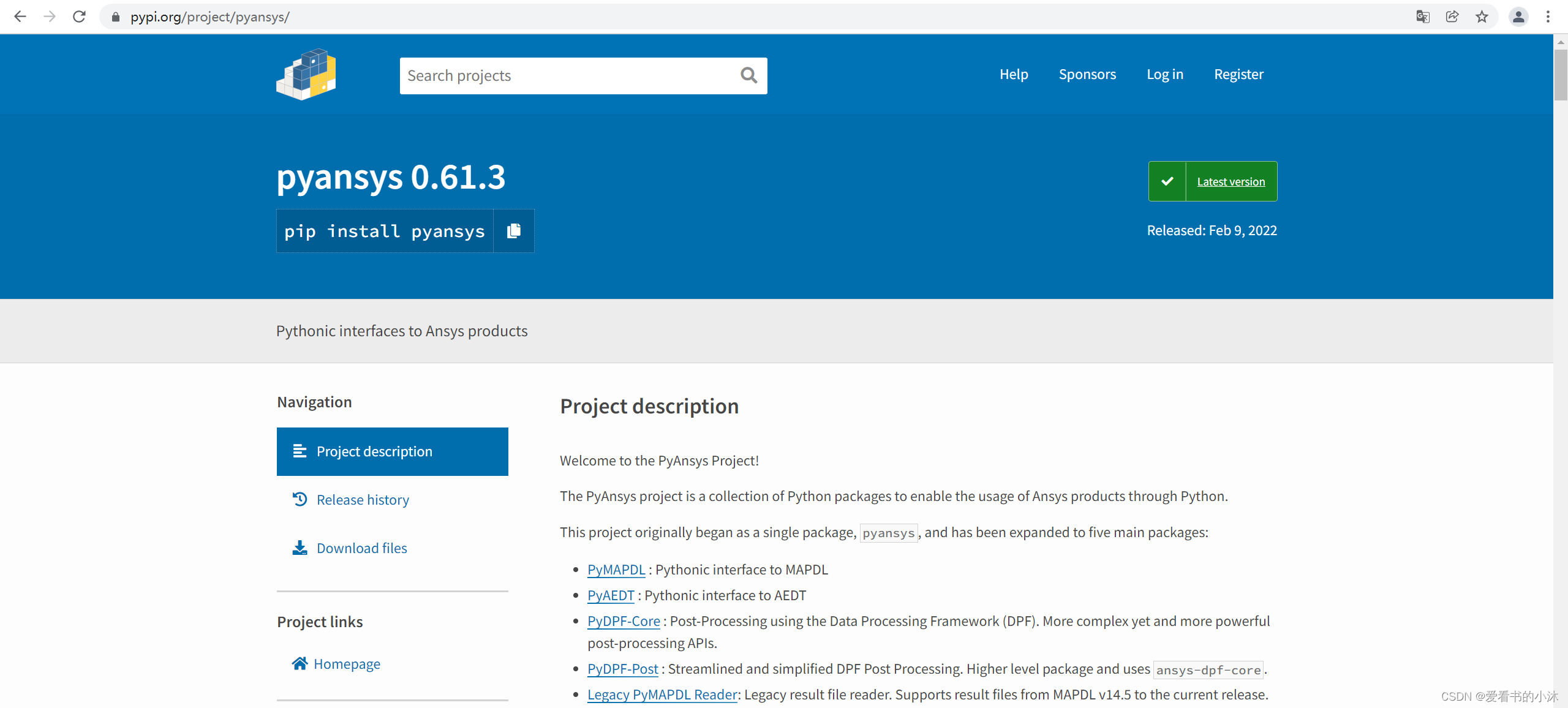
pip install pyansys
pip install pyvista
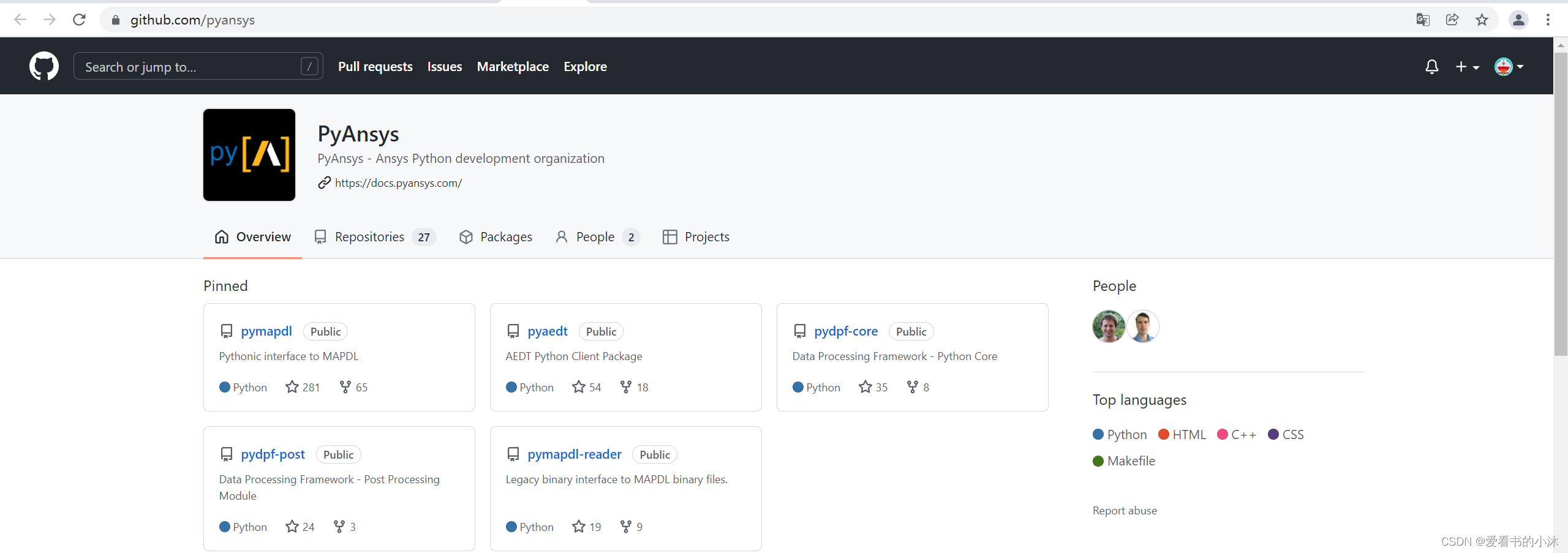
1.2 PyAnsys Project(recommended)
https://docs.pyansys.com/
https://github.com/pyansys

This is the legacy module for reading in binary and ASCII files generated from MAPDL.
This Python module allows you to extract data directly from binary ANSYS v14.5+ files and to display or animate them rapidly using a straightforward API coupled with C libraries based on header files provided by ANSYS.
To use PyAnsys you need to install the applicable packages for your product:
- MAPDL:
pip install ansys-mapdl-core
- AEDT:
pip install pyaedt
- MAPDL Post-Processing:
pip install ansys-dpf-core
pip install ansys-dpf-post
pip install ansys-mapdl-reader
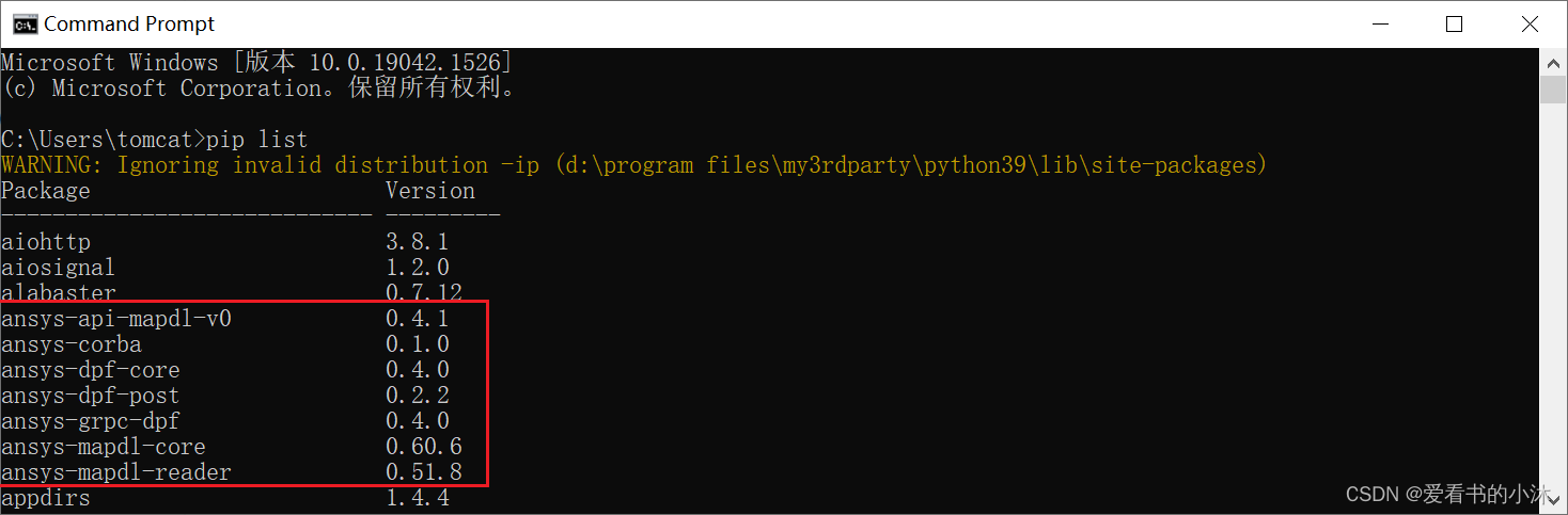
2、安装PyAnsys
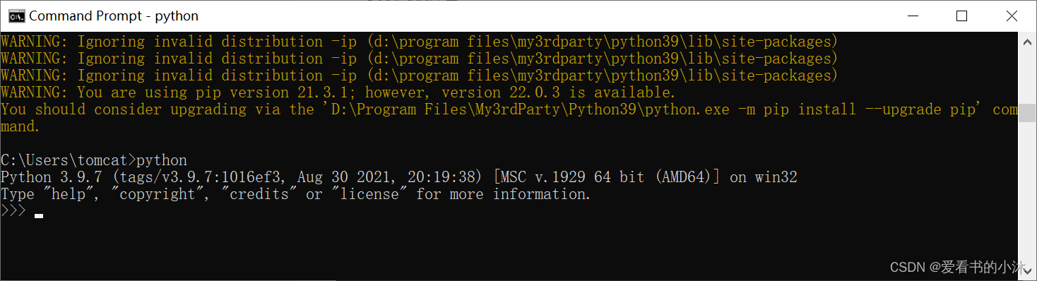
这里测试环境是:
- Win10 x64位,
- Python 3.9.7 x64位,
- VsCode代码编辑器。
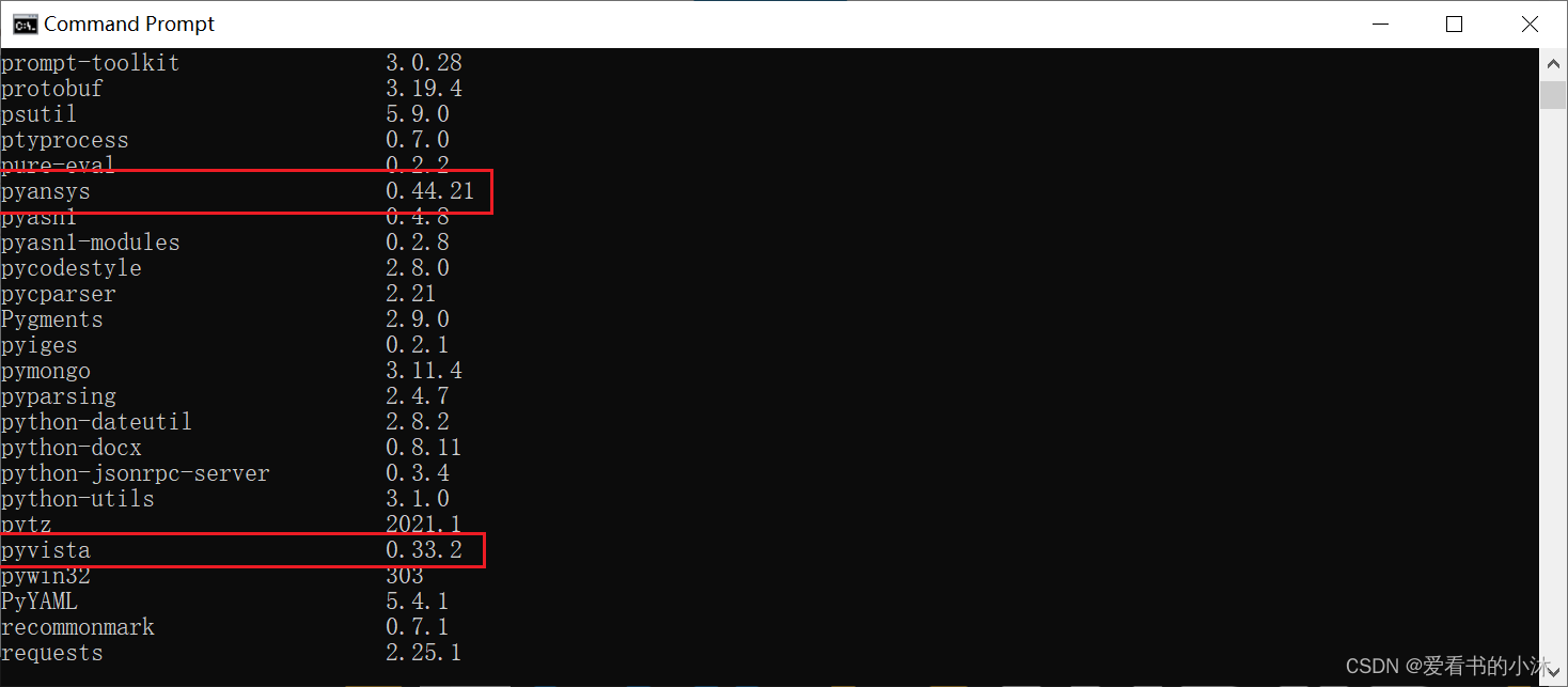
这个项目最初是作为一个单独的包开始的pyansys,并且已经扩展到五个主要包:
- PyMAPDL:MAPDL 的 Pythonic 接口
- PyAEDT : AEDT 的 Pythonic 接口
- PyDPF-Core:使用数据处理框架 (DPF) 进行后处理。更复杂但更强大的后处理 API。
- PyDPF-Post:流线型和简化的 DPF 后处理。更高级别的包和用途ansys-dpf-core。
- Legacy PyMAPDL Reader:旧版结果文件阅读器。支持从 MAPDL v14.5 到当前版本的结果文件。
2.1 PyMAPDL
- 安装此软件包:
pip install ansys-mapdl-core
- All the features of the original module (e.g. pythonic commands, interactive sessions).
- Remote connections to MAPDL from anywhere via gRPC.
- Direct access to MAPDL arrays, meshes, and geometry as Python objects.
- Low level access to the MAPDL solver through APDL math in a scipy like interface.
- 直接从 Python 与 MAPDL 进程进行通信。
from ansys.mapdl.core import launch_mapdl
mapdl = launch_mapdl()
print(mapdl)
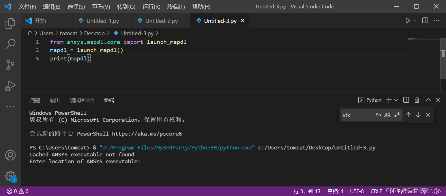
Cached ANSYS executable not found
Enter location of ANSYS executable:
提示:输出信息说明这个子库的功能需要电脑上安装ANSYS软件。
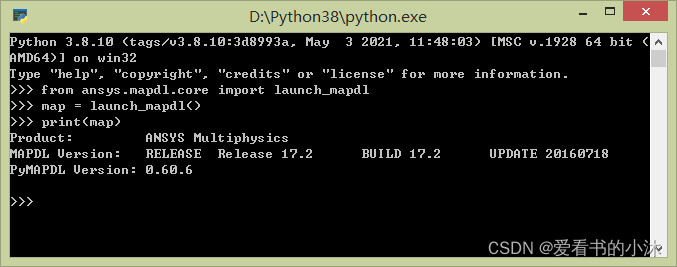
- 补充1:
在一台Win8.1 64位的计算机上安装了Python3.8、Ansys17.2版本之后,子库“ansys-mapdl-core”测试脚本运行通过,截图如下:
- 补充2:
(1)“The ansys-mapdl-core package currently supports Python 3.6 through Python 3.8 on Windows, Mac OS, and Linux.”
(2)“You will need a local licenced copy of ANSYS to run MAPDL prior and including 2021R1. If you have the latest version of 2021R1 you do not need MAPDL installed locally and can connect to a remote instance via gRPC.”
以上(1)、(2)两段文字来自官网:https://pypi.org/project/ansys-mapdl-core/
2.2 PyAEDT
- 安装此软件包:
pip install pyaedt
2.3 PyDPF-Core
- 安装此软件包:
pip install ansys-dpf-core
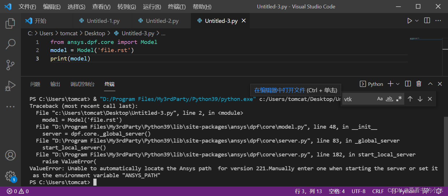
ValueError: Unable to automatically locate the Ansys path for version 221.Manually enter one when starting the server or set it as the environment variable “ANSYS_PATH”
提示:输出信息说明这个子库的功能需要电脑上安装ANSYS软件。
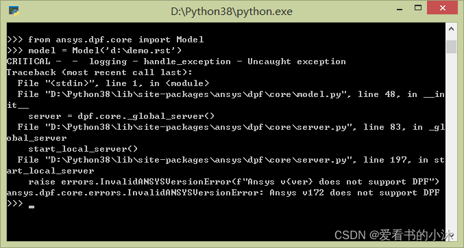
- 补充1:
在一台Win8.1 64位的计算机上安装了Python3.8、Ansys17.2版本之后,子库“ansys-dpf-core”和“ansys-dpf-post”测试脚本运行失败,截图如下:
- 补充2:
“Provided you have ANSYS 2021R1 or higher installed, a DPF server will start automatically once you start using DPF.”
以上这段文字来自官网:https://pypi.org/project/ansys-dpf-core/
2.4 PyDPF-Post
- 安装此软件包:
pip install ansys-dpf-post
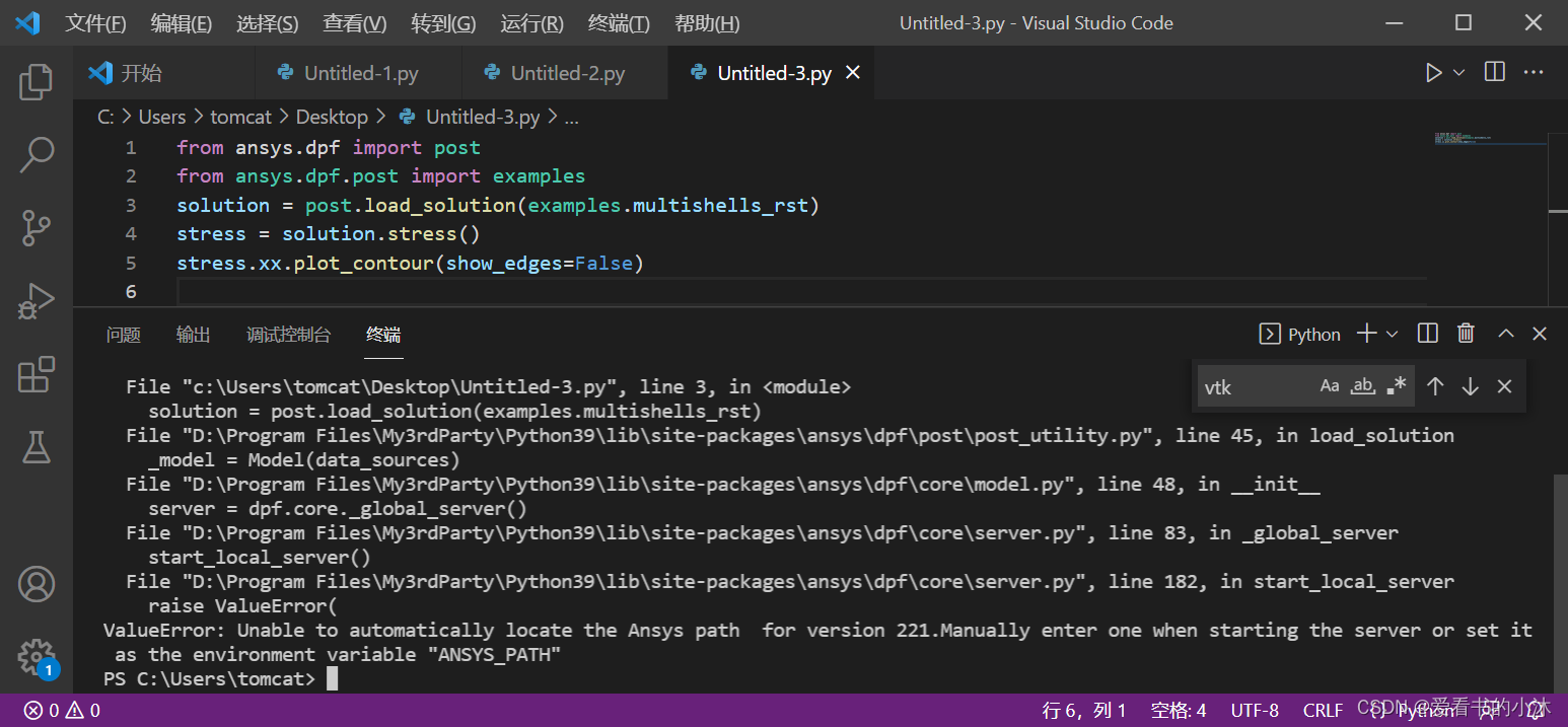
ValueError: Unable to automatically locate the Ansys path for version 221.Manually enter one when starting the server or set it as the environment variable “ANSYS_PATH”
提示:输出信息说明这个子库的功能需要电脑上安装ANSYS软件。
- 补充1:
“Provided you have ANSYS 2021R1 installed, a DPF server will start automatically once you start using DPF-Post. Should you wish to use DPF-Post without 2020R1, see the DPF Docker documentation.”
以上这段文字来自官网:https://pypi.org/project/ansys-dpf-post/
2.5 Legacy PyMAPDL Reader
This module will likely change or be depreciated in the future.
You are encouraged to use the new Data Processing Framework (DPF) modules at DPF-Core and DPF-Post as they provide a modern interface to ANSYS result files using a client/server interface using the same software used within ANSYS Workbench, but via a Python client.
- 安装此软件包:
pip install ansys-mapdl-reader
测试代码如下:
- 过时的写法:
import pyansys
from pyansys import examples

rst = pyansys.read_binary(examples.rstfile)

freqs = rst.time_values
print(freqs)

print(rst.mesh)
print(rst.mesh.nnum)
print(rst.mesh.enum)
rst.plot_nodal_solution(0)
rst.plot_nodal_solution(1)
rst.plot_nodal_solution(2)
rst.plot_nodal_solution(3)
rst.plot_nodal_solution(4)
rst.plot_nodal_solution(5)
- 推荐的写法:
from ansys.mapdl import reader as pymapdl_reader
from ansys.mapdl.reader import examples

# Sample result file
rstfile = examples.rstfile

# Create result object by loading the result file
result = pymapdl_reader.read_binary(rstfile)

result.plot_nodal_solution(0)
result.plot_nodal_solution(1)
result.plot_nodal_solution(2)
result.plot_nodal_solution(3)
result.plot_nodal_solution(4)
result.plot_nodal_solution(5)
运行没有报错!!!
提示:输出信息说明这个子库的功能不需要电脑上安装ANSYS软件!!!
(1)这是用于读取从 MAPDL 生成的二进制和 ASCII 文件的遗留模块。
这个 Python 模块允许您直接从二进制 ANSYS v14.5+ 文件中提取数据,并使用简单的 API 以及基于 ANSYS 提供的头文件的 C 库快速显示或动画化它们。
(2)该模块将来可能会更改或废弃。
我们鼓励您在DPF-Core和 DPF-Post上查看新的数据处理框架 (DPF) 模块,因为它们使用客户端/服务器接口为 ANSYS 结果文件提供现代接口使用 ANSYS Workbench 中使用的相同软件,但通过 Python 客户端。
- 补充1:
(1)“This is the legacy module for reading in binary and ASCII files generated from MAPDL.
This Python module allows you to extract data directly from binary ANSYS v14.5+ files and to display or animate them rapidly using a straightforward API coupled with C libraries based on header files provided by ANSYS.”
(2)“PyMAPDL-Reader requires the VTK library which, at the moment, is not available for Python 3.10 in their official channel. If you wish to install PyMAPDL-Reader in Python 3.10, you can still do it by using the unofficial VTK wheel from PyVista using –find-links. This tells pip to look for vtk at wheels.pyvista.org. ”
以上(1)、(2)这两段文字来自官网:https://pypi.org/project/ansys-mapdl-reader/
下面章节就使用ansys-mapdl-reader子库测试相关功能。
3、官网入门示例
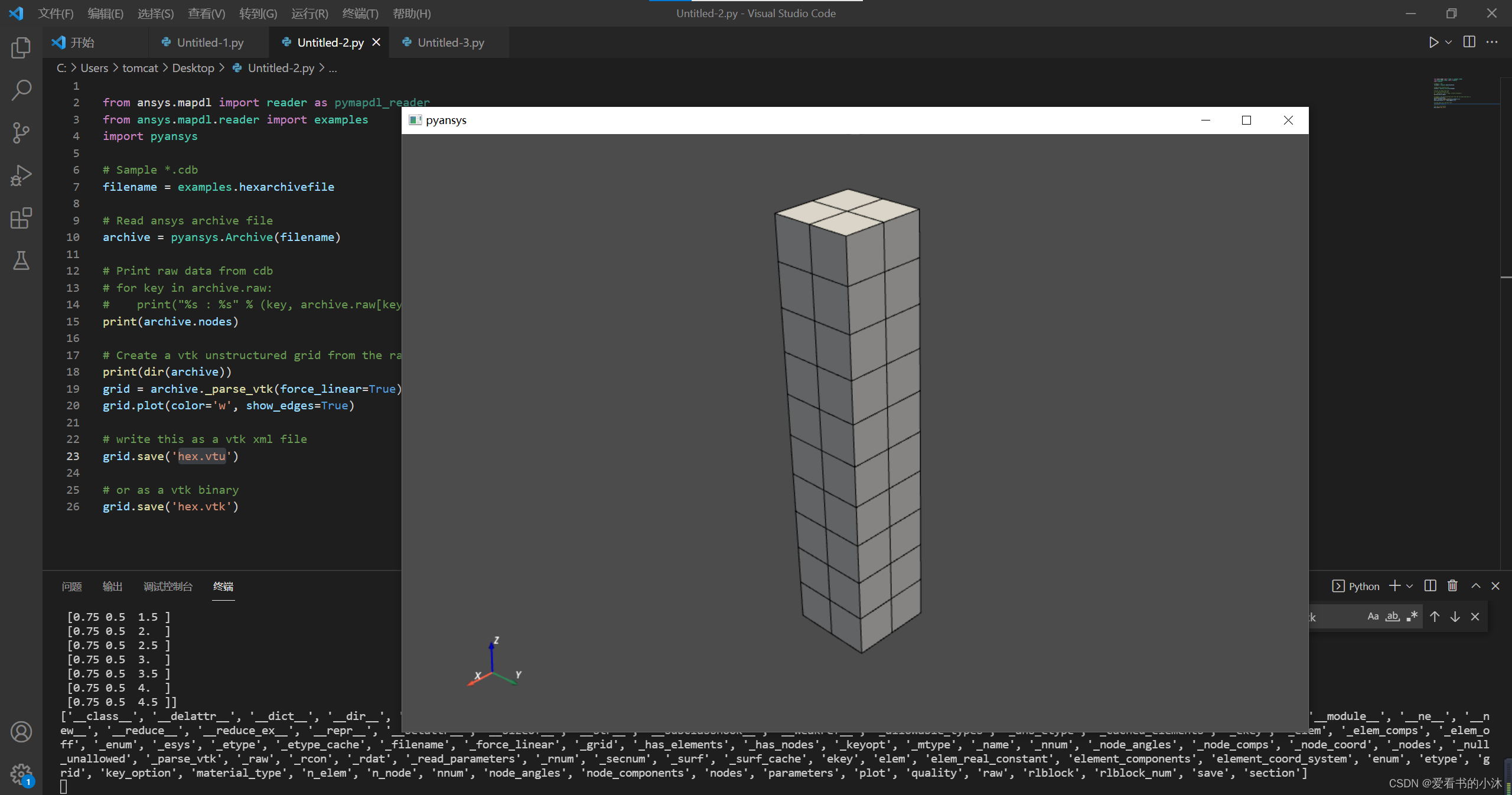
3.1 Loading and Plotting an Ansys Archive File
ANSYS archive files containing solid elements (both legacy and modern), can be loaded using Archive and then converted to a vtk object.
from ansys.mapdl import reader as pymapdl_reader
from ansys.mapdl.reader import examples
import pyansys

# Sample *.cdb
filename = examples.hexarchivefile

# Read ansys archive file
archive = pyansys.Archive(filename)

# Print raw data from cdb
# for key in archive.raw:
#    print("%s : %s" % (key, archive.raw[key]))
print(archive.nodes)

# Create a vtk unstructured grid from the raw data and plot it
print(dir(archive))
grid = archive._parse_vtk(force_linear=True)
grid.plot(color='w', show_edges=True)

# write this as a vtk xml file
grid.save('hex.vtu')

# or as a vtk binary
grid.save('hex.vtk')
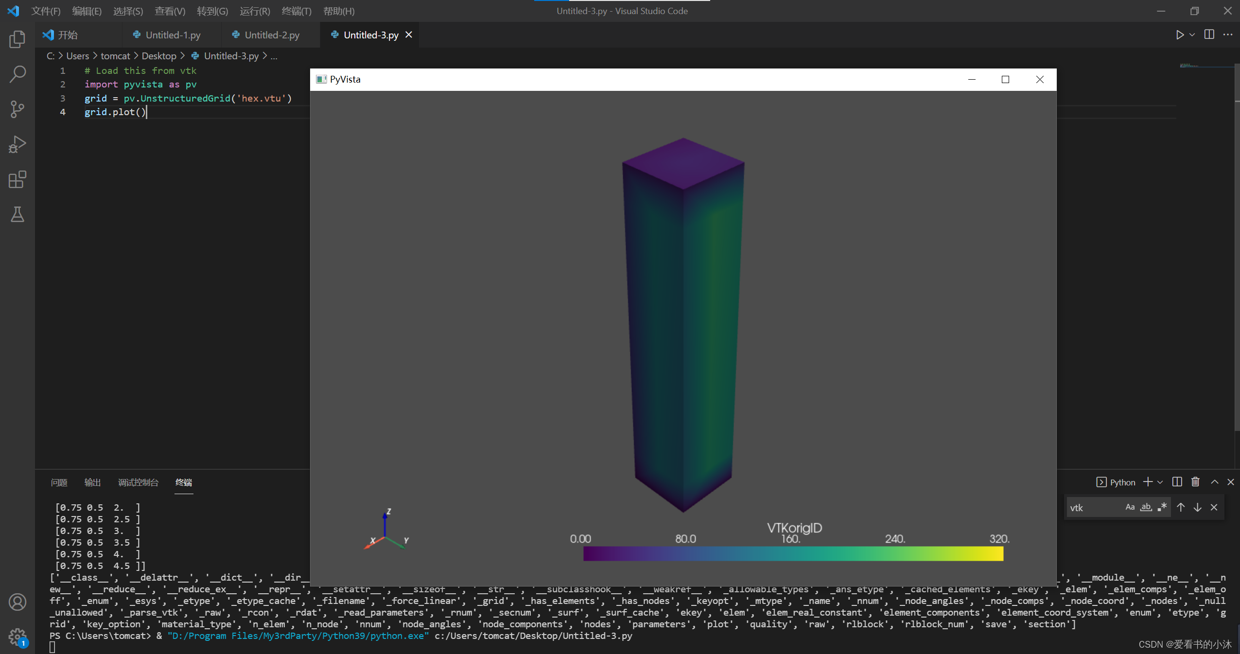
3.2 Loading vtk file by using pyvista
You can then load this vtk file using pyvista or another program that uses VTK.
# Load this from vtk
import pyvista as pv
grid = pv.UnstructuredGrid('hex.vtu')
grid.plot()
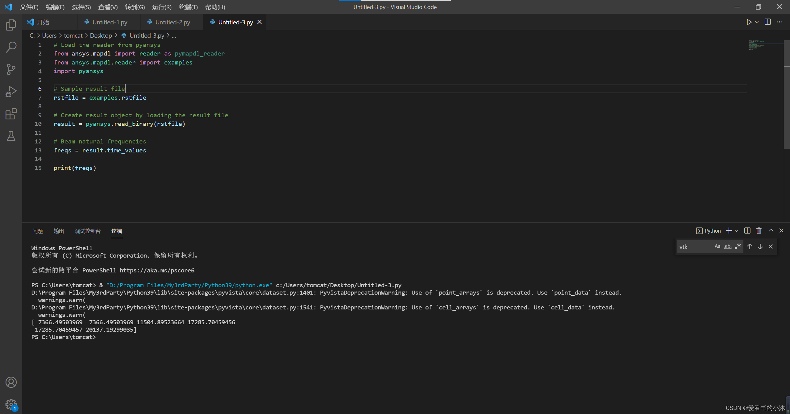
3.3 Loading the Result File
This example reads in binary results from a modal analysis of a beam from MAPDL.
from ansys.mapdl import reader as pymapdl_reader
from ansys.mapdl.reader import examples

# Sample result file
rstfile = examples.rstfile

# Create result object by loading the result file
result = pymapdl_reader.read_binary(rstfile)

# Beam natural frequencies
freqs = result.time_values

print(freqs)
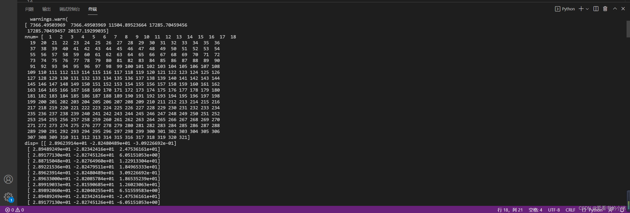
3.4 Listing Nodal Results
Get the 1st bending mode shape. Results are ordered based on the sorted node numbering. Note that results are zero indexed
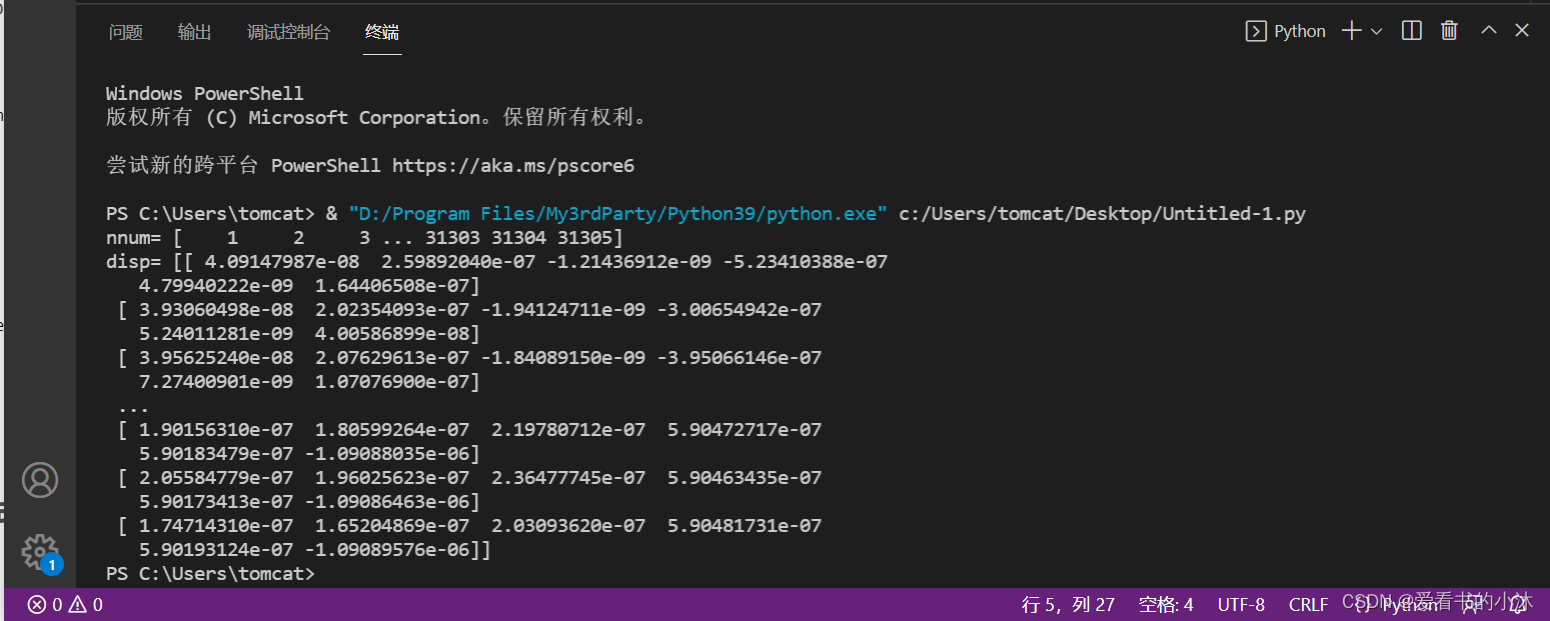
nnum, disp = result.nodal_solution(0)
print("nnum=", nnum)
print("disp=", disp)
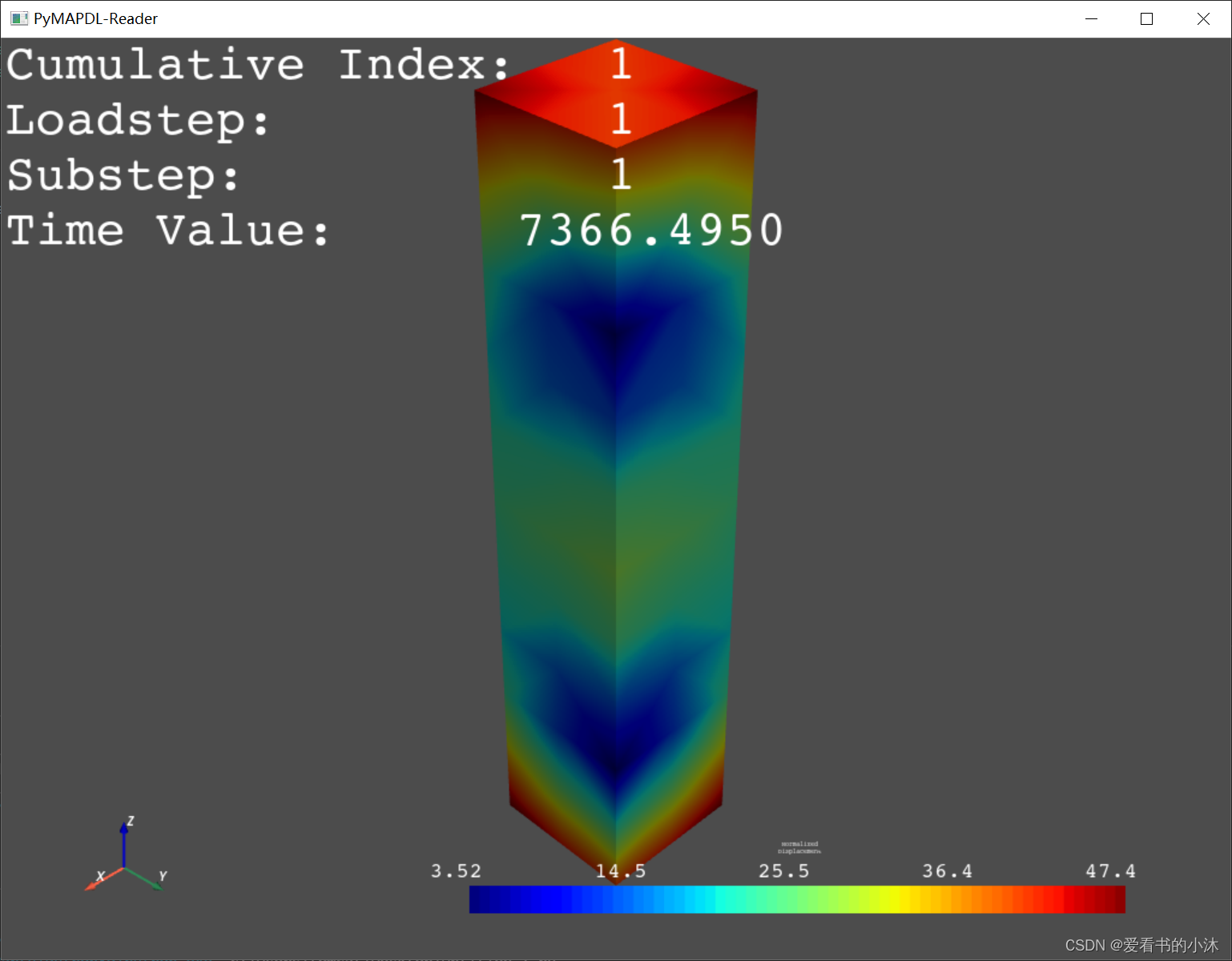
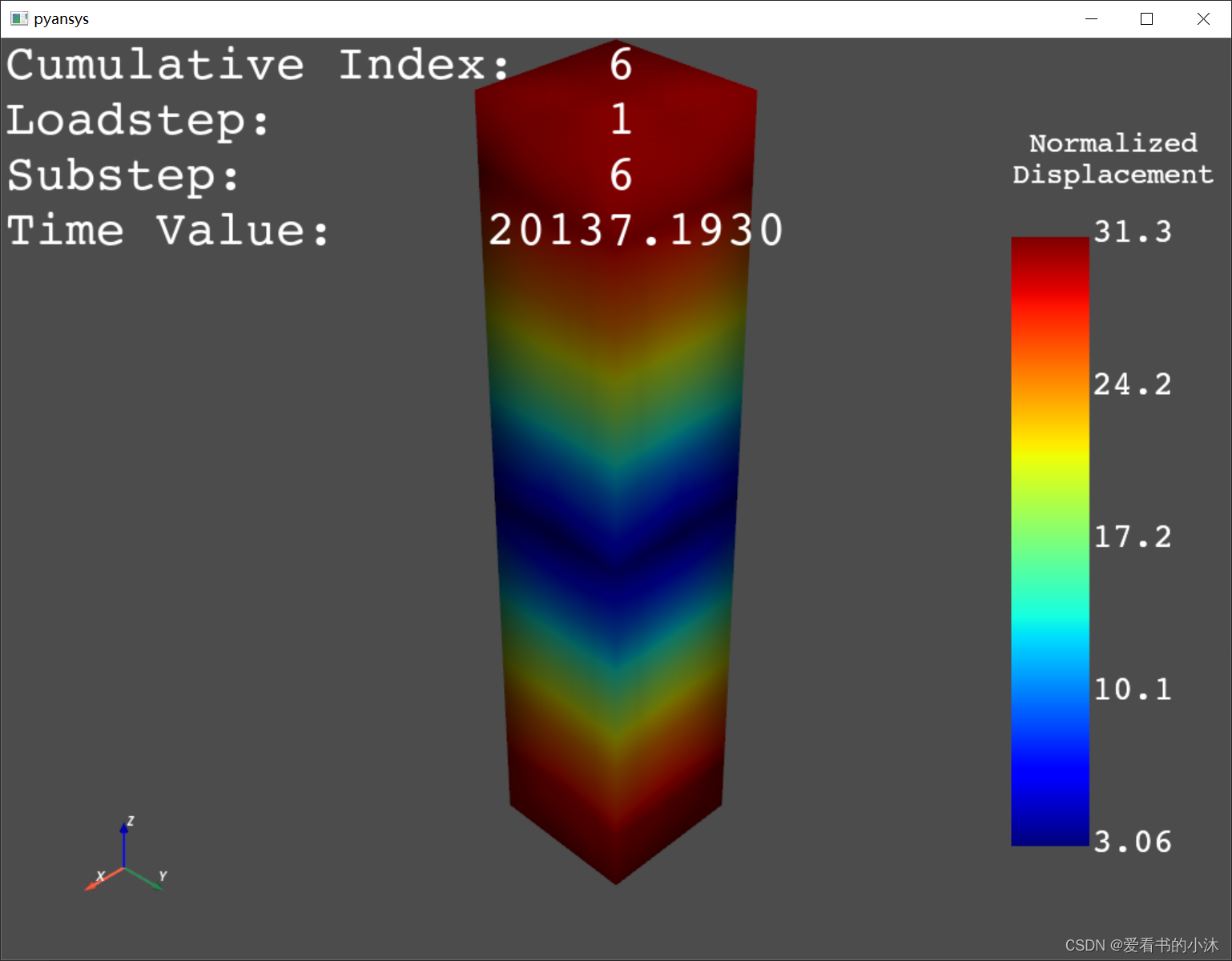
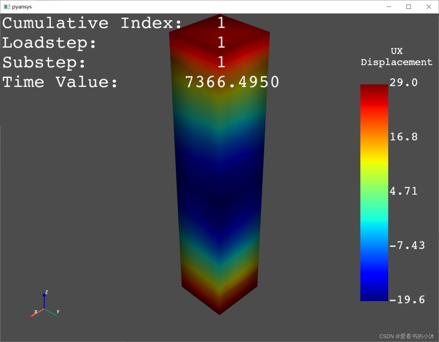
3.5 Plotting Nodal Results(Solution)
# Plot the displacement of Mode 0 in the x direction
result.plot_nodal_solution(0, 'x', label='Displacement')
First, get the camera position from an interactive plot:
cpos=None
result.plot_nodal_solution(0, 'x', label='Displacement', cpos=cpos,
                           screenshot='hexbeam_disp.png',
                           window_size=[800, 600], interactive=False)
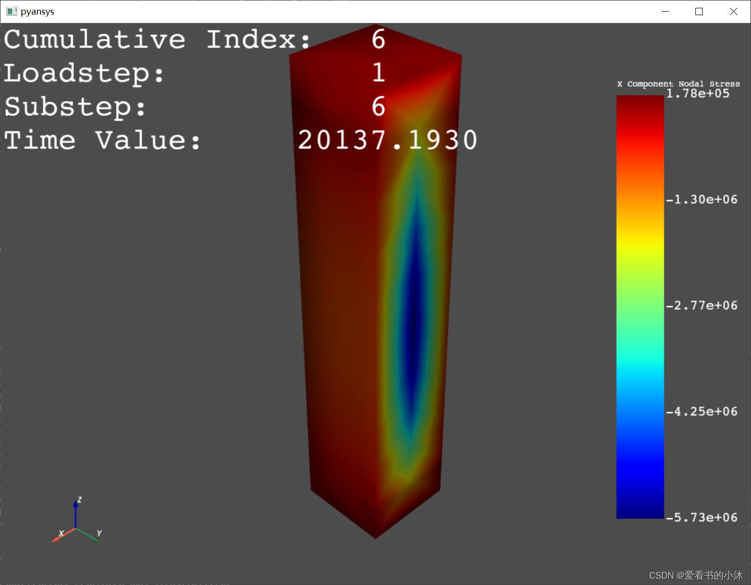
3.6 Plotting Nodal Results(Stress)
Stress can be plotted as well using the below code. The nodal stress is computed in the same manner that Ansys uses by to determine the stress at each node by averaging the stress evaluated at that node for all attached elements. For now, only component stresses can be displayed.
Please select from the following: [‘X’, ‘Y’, ‘Z’, ‘XY’, ‘YZ’, ‘XZ’]
# Display node averaged stress in x direction for result 6
result.plot_nodal_stress(5, 'X')
3.7 Animating Nodal Results
result.animate_nodal_solution(0, loop=False, movie_filename='result.gif',
                             background='grey', displacement_factor=0.01, show_edges=True,
                             add_text=True,
                             n_frames=30)
4、官网进阶示例
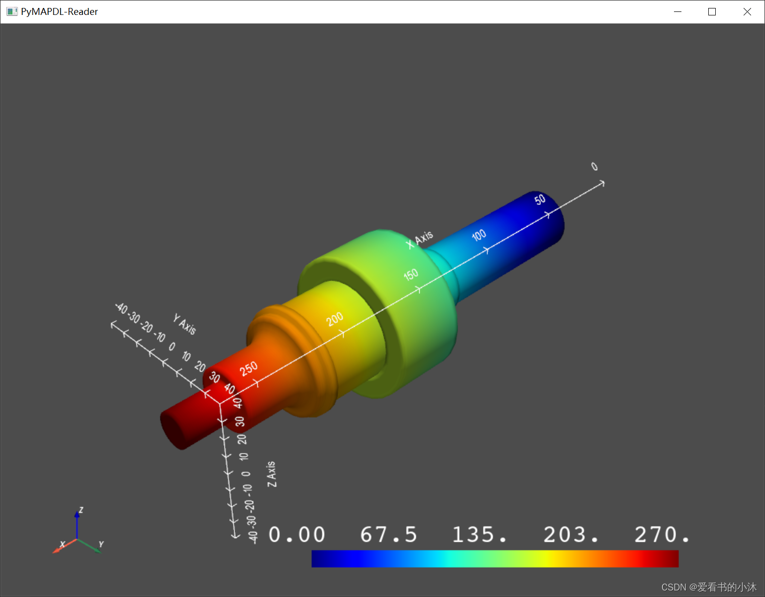
4.1 Custom Scalar Visualization(自定义标量可视化)
- 绘制节点标量
import pyvista
import numpy as np

from ansys.mapdl import reader as pymapdl_reader
from ansys.mapdl.reader import examples

# Download an example shaft modal analysis result file
shaft = examples.download_shaft_modal()

print('shaft.mesh:\n', shaft.mesh)
print('-'*79)
print('shaft.grid:\n', shaft.grid)

## plot one
# shaft.grid.plot(color='w', smooth_shading=True)

## plot two
x_scalars = shaft.grid.points[:, 0]
shaft.grid.plot(scalars=x_scalars, smooth_shading=True)
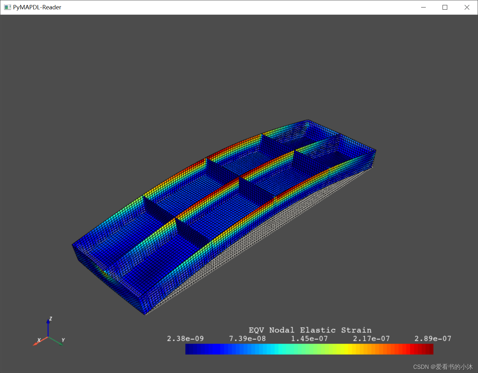
- 绘制缺失值
import pyvista
import numpy as np

from ansys.mapdl import reader as pymapdl_reader
from ansys.mapdl.reader import examples

pontoon = examples.download_pontoon()
nnum, strain = pontoon.nodal_elastic_strain(0)

scalars = strain[:, 0]
scalars[:2000] = np.nan  # here, we simulate unknown values

pontoon.grid.plot(scalars=scalars, show_edges=True, lighting=False)
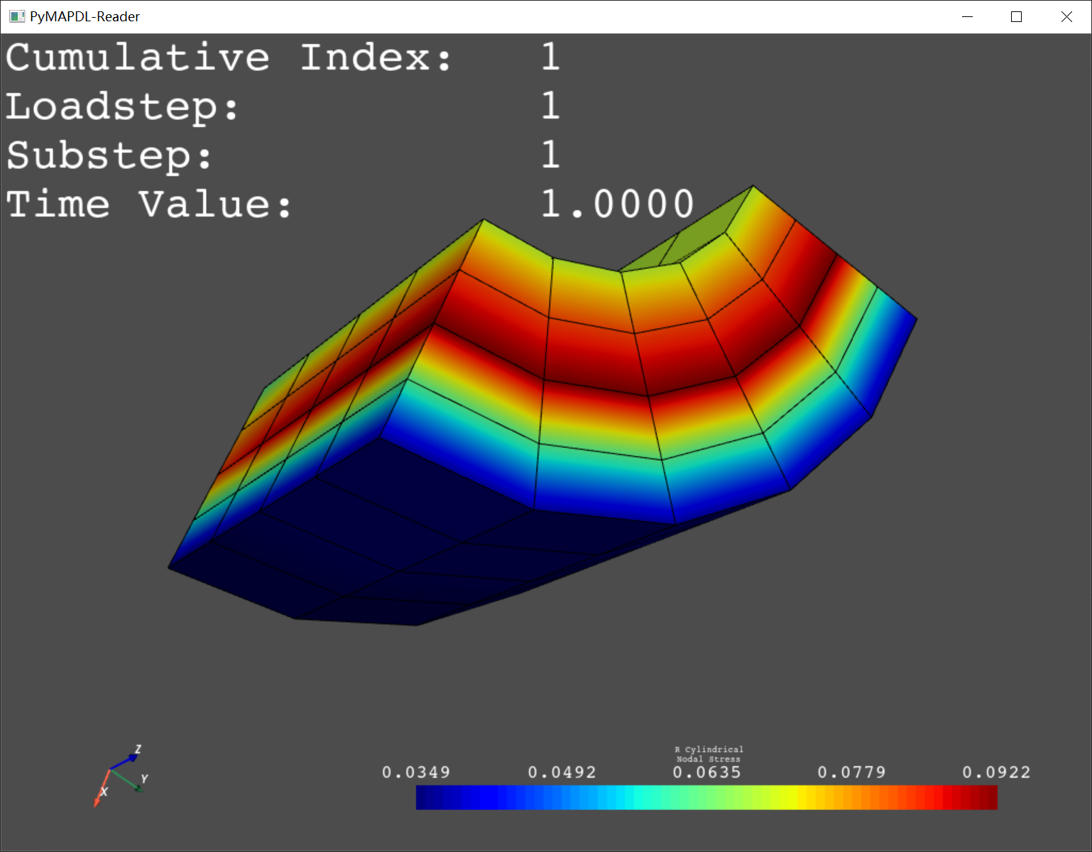
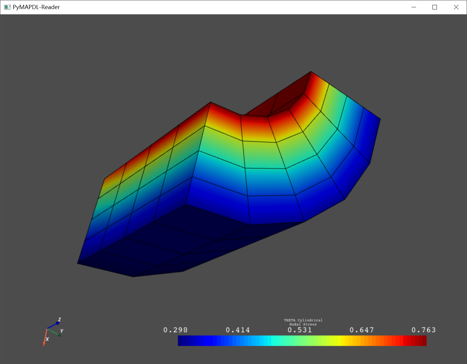
4.2 Cylindrical Nodal Stress(圆柱节点应力)
圆柱节点应力:可视化径向上的节点应力。这相当于在 MAPDL 中将结果坐标系设置为圆柱体。
from ansys.mapdl.reader import examples
rst = examples.download_corner_pipe()
# obtain the cylindrical_nodal_stress
nnum, stress = rst.cylindrical_nodal_stress(0)
print(stress)
# contains results for each node in following directions
# R, THETA, Z, RTHETA, THETAZ, and RZ
print(stress.shape)
## 绘制径向上的圆柱节点应力
# _ = rst.plot_cylindrical_nodal_stress(0, 'R', show_edges=True, show_axes=True)
## 在 theta 方向绘制圆柱节点应力
# _ = rst.plot_cylindrical_nodal_stress(0, 'THETA', show_edges=True, show_axes=True,
# add_text=False)
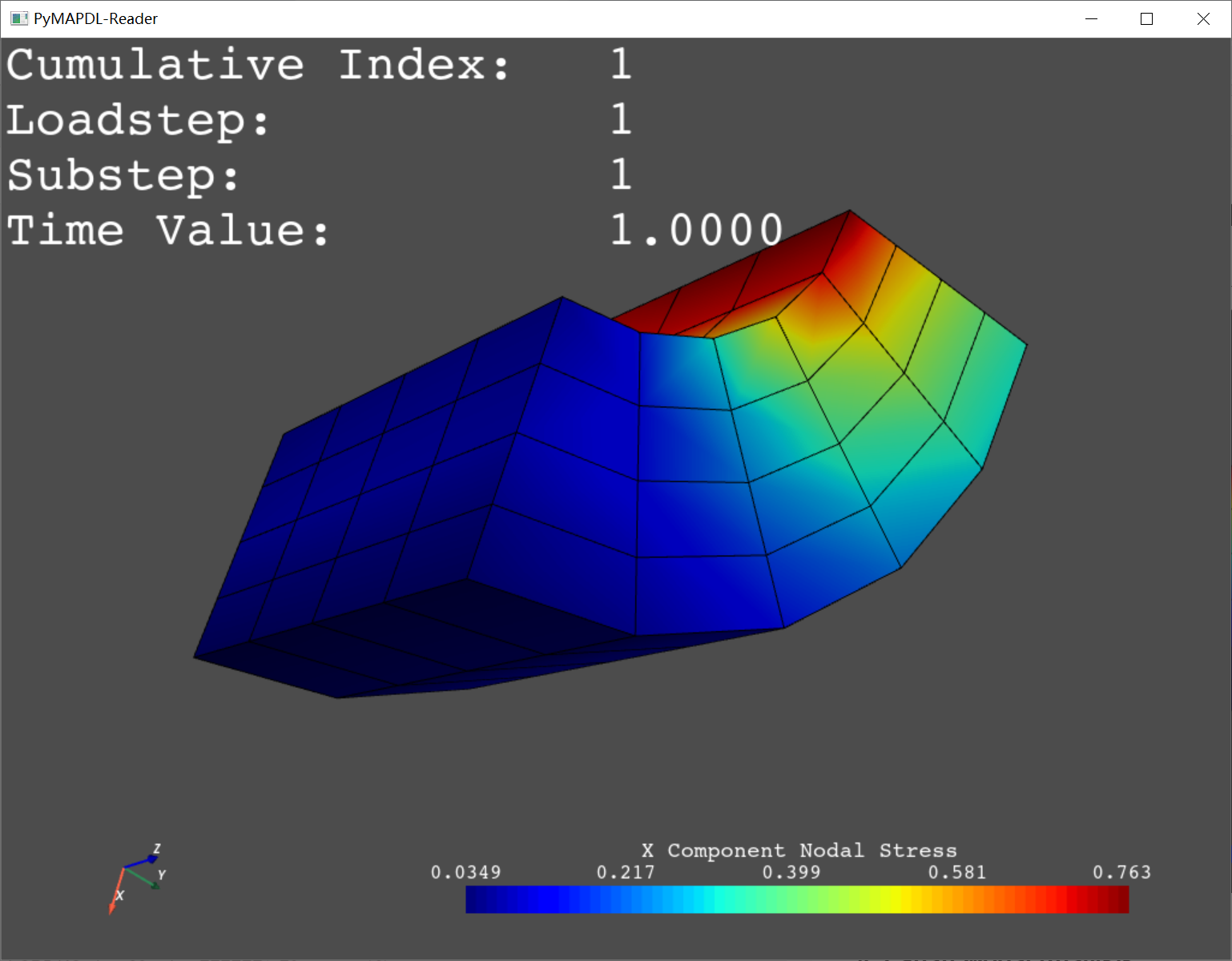
## 在“X”方向绘制笛卡尔应力
_ = rst.plot_nodal_stress(0, 'X', show_edges=True, show_axes=True)
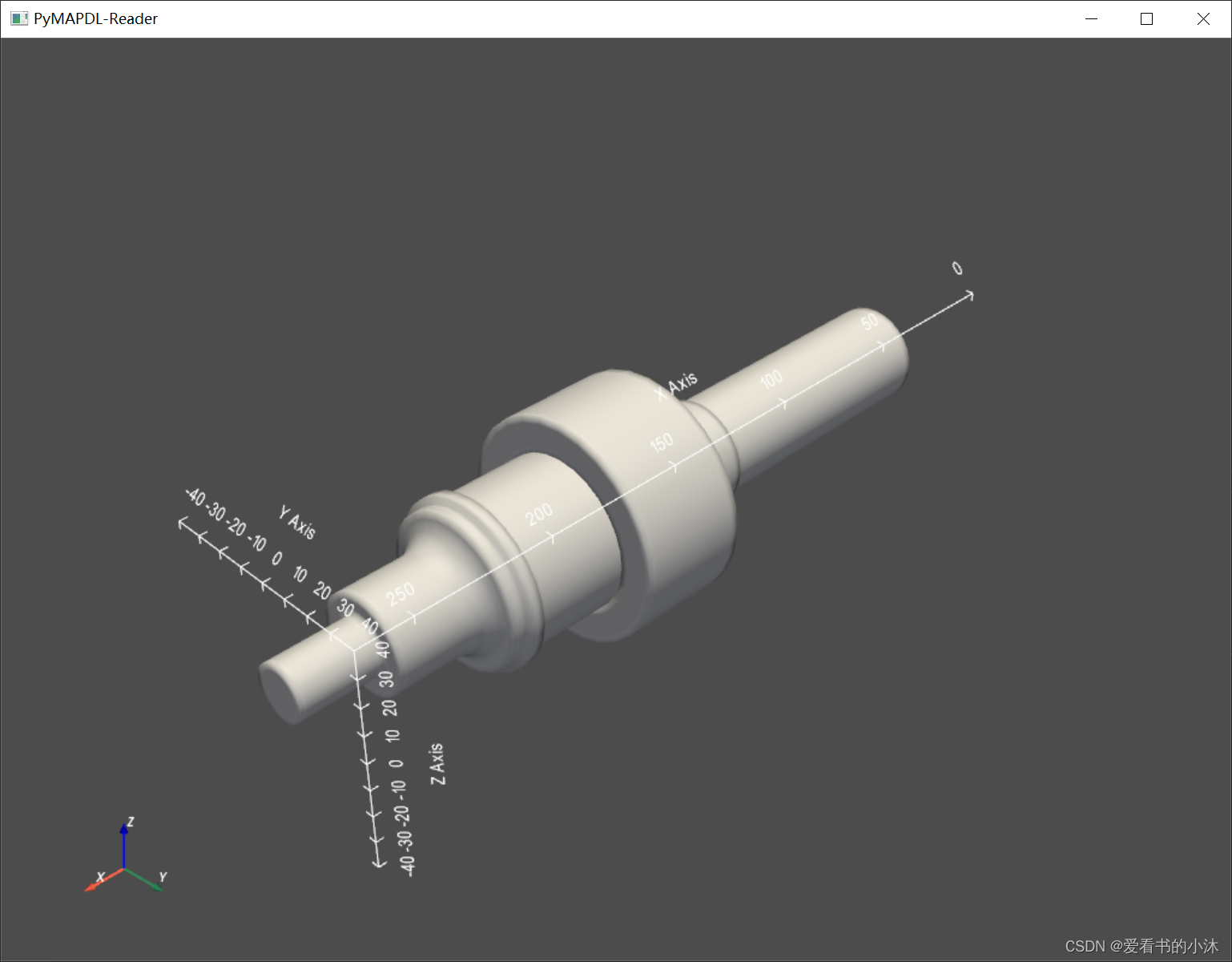
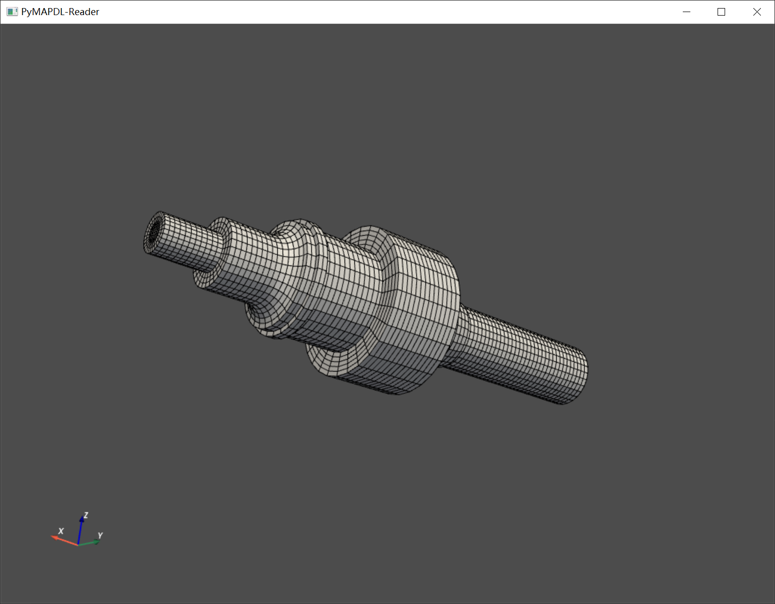
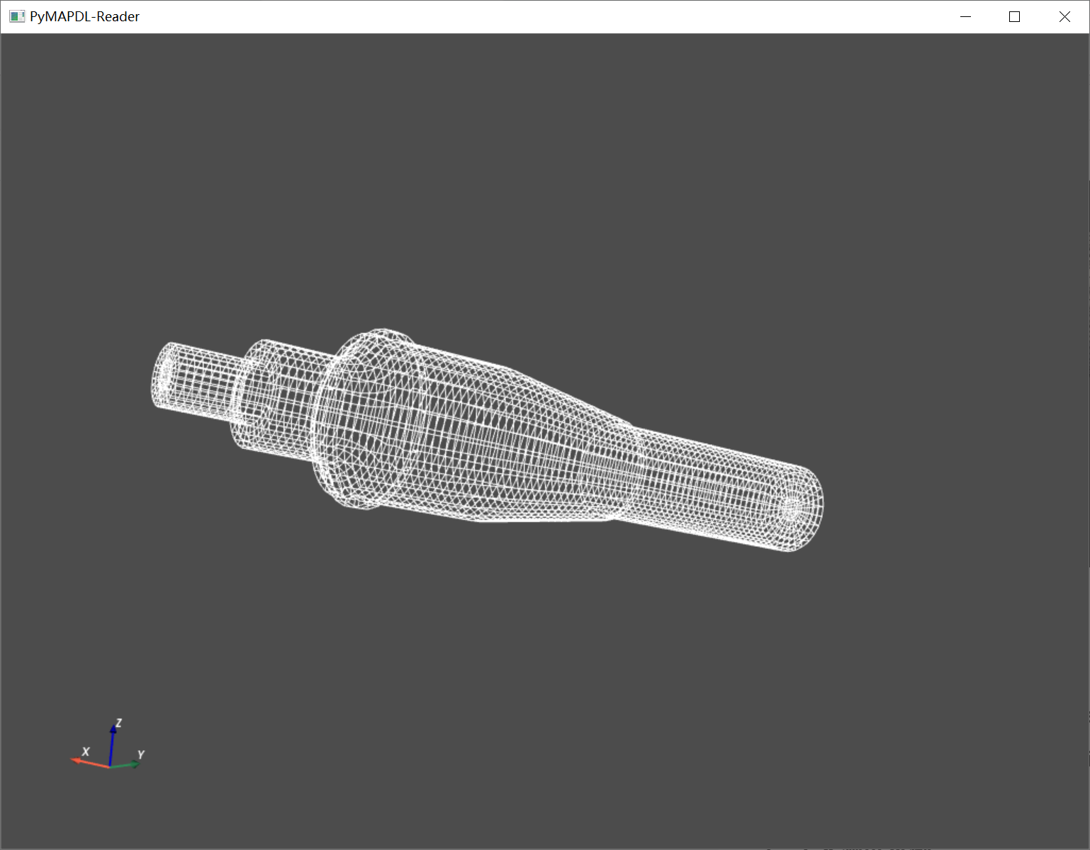
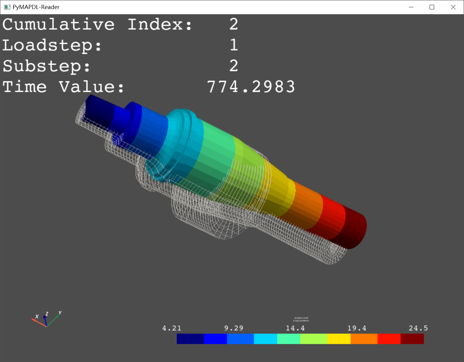
4.3 Shaft Modal Analysis(可视化轴模态分析)
# sphinx_gallery_thumbnail_number = 6
from ansys.mapdl.reader import examples
# Download an example shaft modal analysis result file
shaft = examples.download_shaft_modal()
print(shaft.mesh)
print(shaft.mesh._grid)
## 绘制节点组件
# cpos = shaft.plot()
cpos = [(-115.35773008378118, 285.36602704380107, -393.9029392590675),
(126.12852038381345, 0.2179228023931401, 5.236408799851887),
(0.37246222812978824, 0.8468424028124546, 0.37964435122285495)]
## 将节点组件绘制为线框
# shaft.plot(element_components=['SHAFT_MESH'], cpos=cpos, style='wireframe',
# lighting=False)
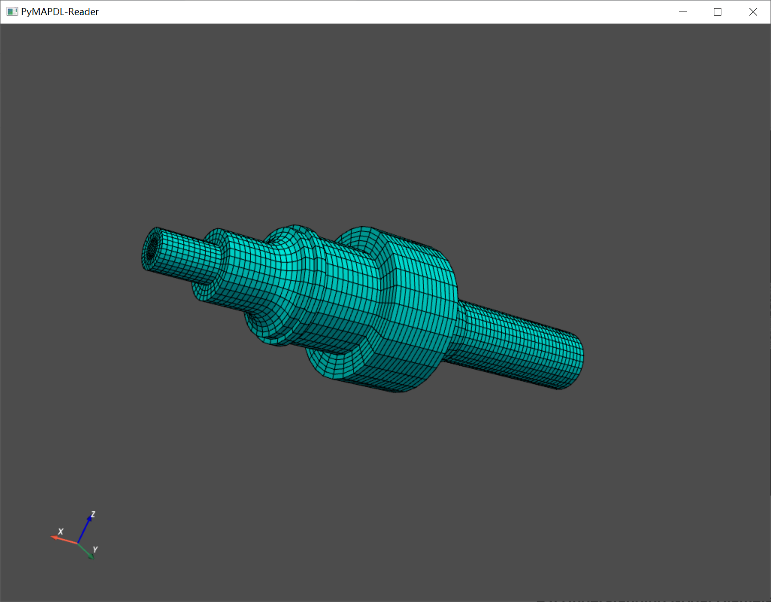
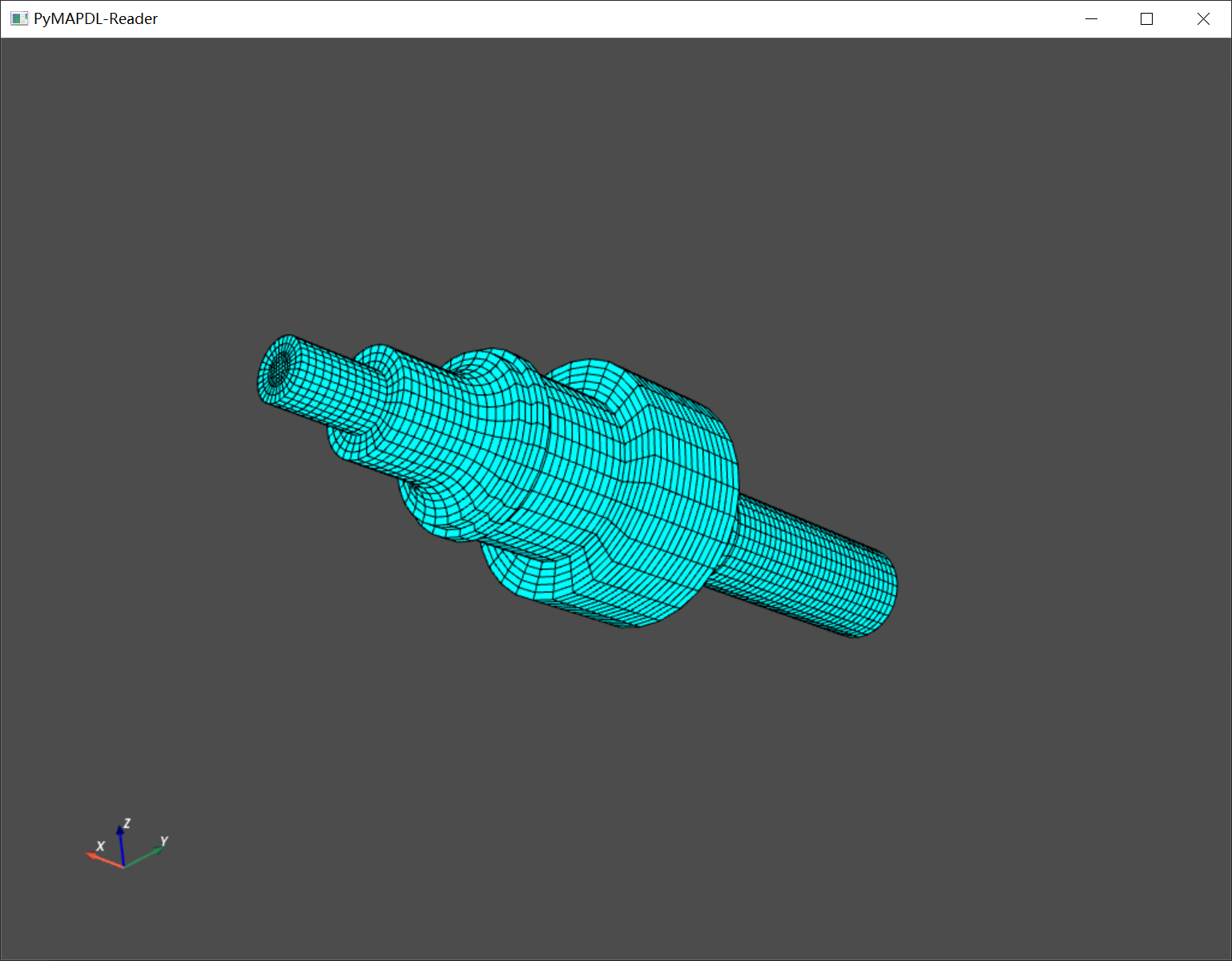
## 绘制带有边缘和蓝色的轴
# shaft.plot(show_edges=True, color='cyan')
## 绘制没有照明但有边缘和蓝色的轴
# shaft.plot(lighting=False, show_edges=True, color='cyan')
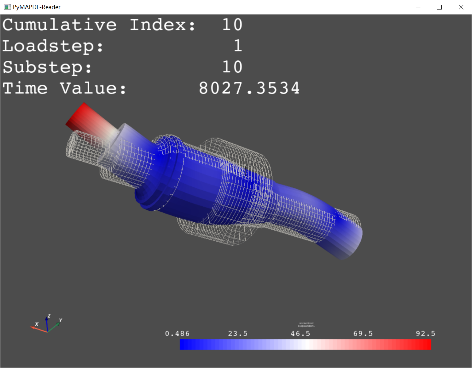
## 使用“bwr”颜色图绘制没有等高线的振型
# shaft.plot_nodal_solution(9, element_components=['SHAFT_MESH'],
# show_displacement=True, cmap='bwr',
# displacement_factor=0.3, stitle=None,
# overlay_wireframe=True, cpos=cpos)
## 绘制带有轮廓和默认颜色图的模式形状
# shaft.plot_nodal_solution(1, element_components=['SHAFT_MESH'],
# n_colors=10, show_displacement=True,
# displacement_factor=1, stitle=None,
# overlay_wireframe=True, cpos=cpos)
## 为轴组件的模式设置动画
shaft.animate_nodal_solution(5, element_components='SHAFT_MESH',
comp='norm', displacement_factor=1,
show_edges=True, cpos=cpos,
loop=False, movie_filename='demo.gif',
n_frames=30)
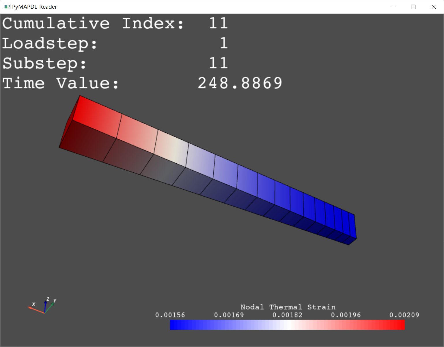
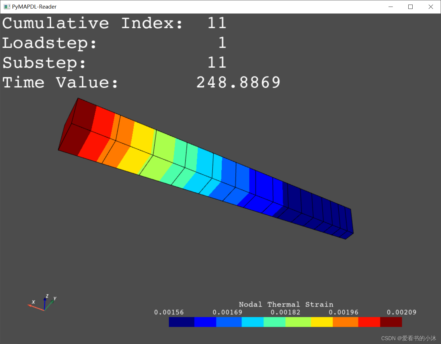
4.4 Thermal Analysis(热分析)
from ansys.mapdl.reader import examples

vm33 = examples.download_verification_result(33)

# get nodal thermal strain for result set 1
nnum, tstrain = vm33.nodal_thermal_strain(0)

# plot nodal thermal strain for result set 11 in the X direction
# vm33.plot_nodal_thermal_strain(10, 'X', show_edges=True,
#                                lighting=True, cmap='bwr', show_axes=True)

## 绘制等高线
# Disable lighting and set number of colors to 10 to make an MAPDL-like plot
#vm33.plot_nodal_thermal_strain(10, 'X', show_edges=True, n_colors=10,
#                               interpolate_before_map=True,
#                               lighting=False, show_axes=True)

vm33.animate_nodal_solution(10, loop=False, movie_filename='vm33.gif',
                             background='grey', comp='norm', displacement_factor=1, show_edges=True,
                             add_text=True,
                             n_frames=30)
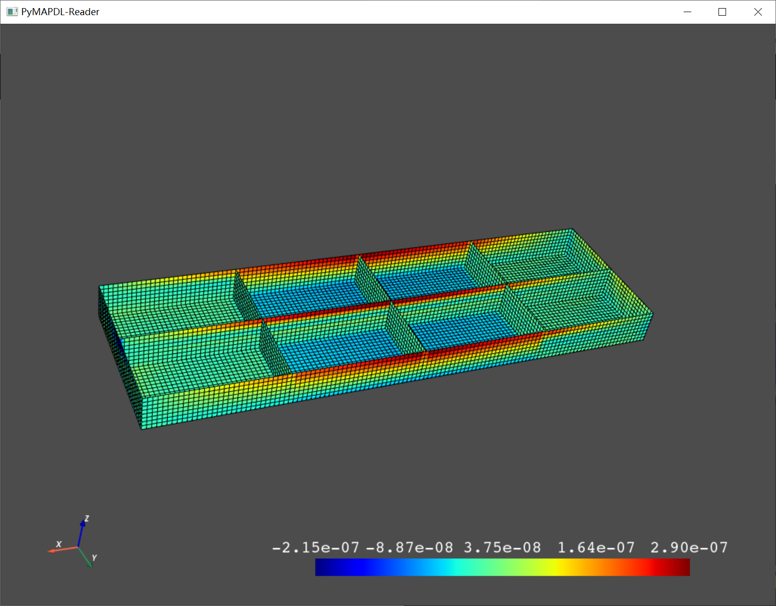
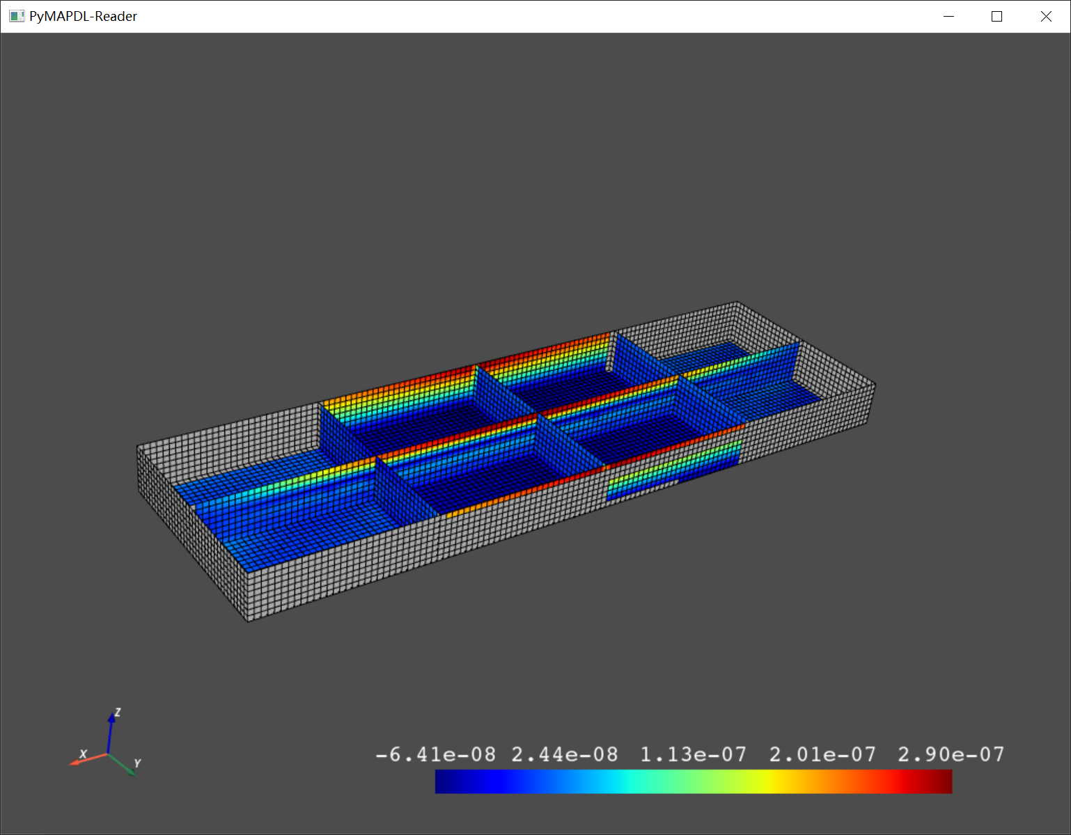
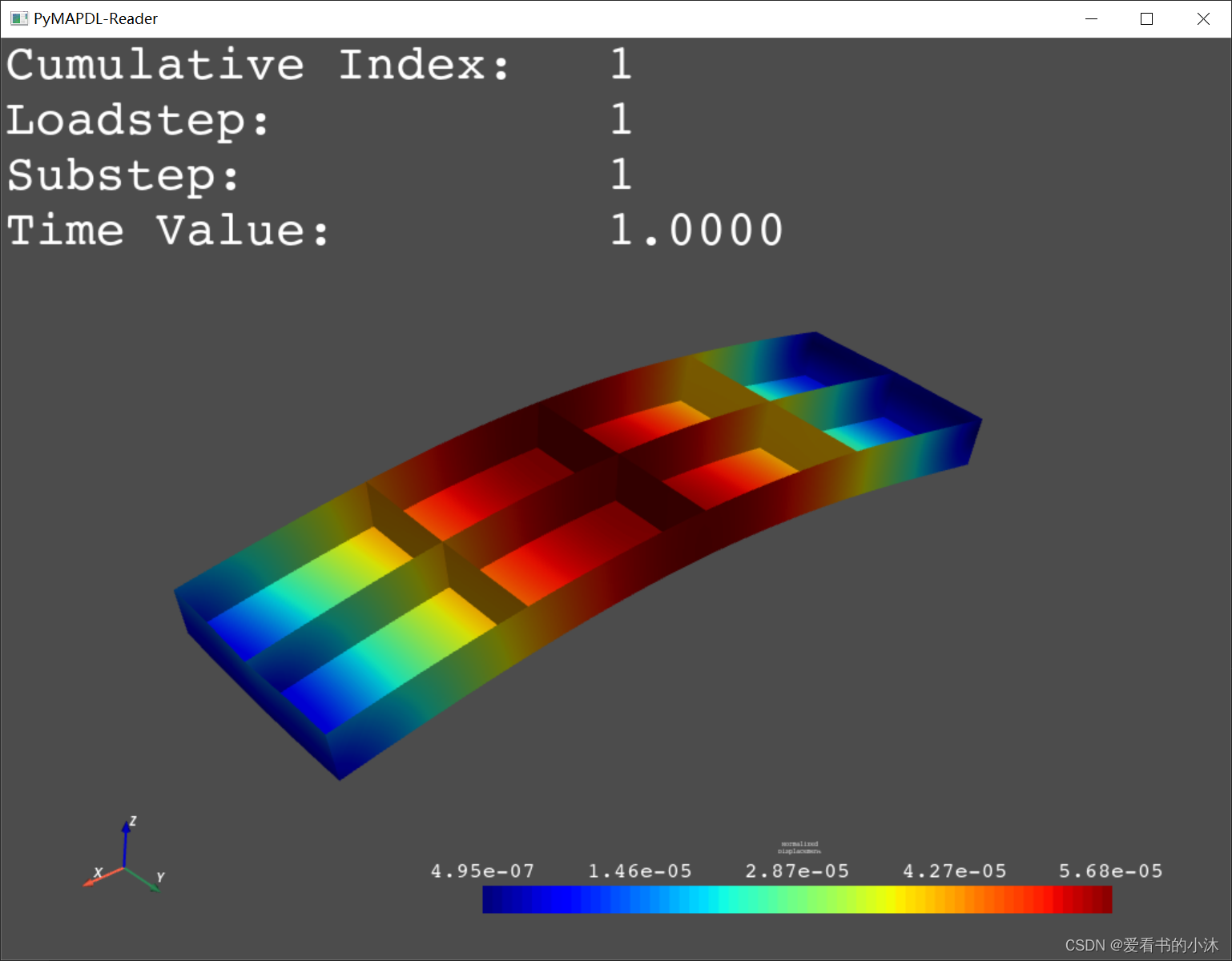
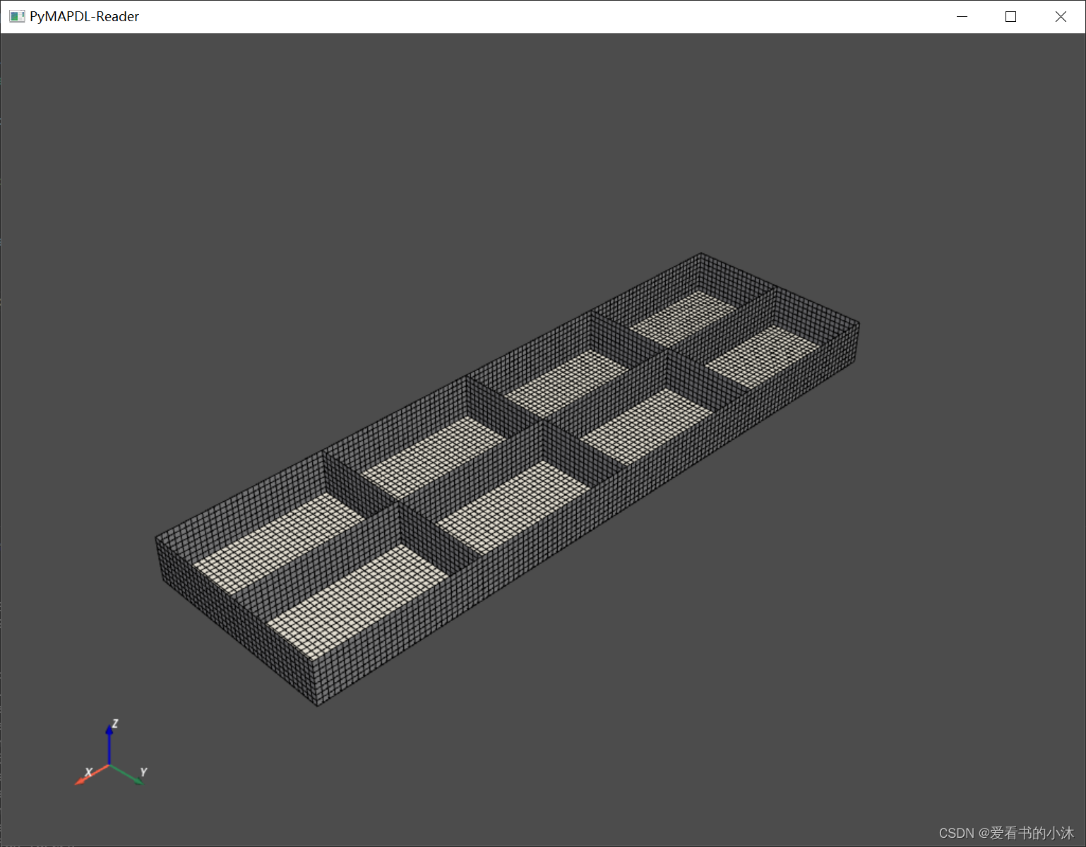
4.5 Shell Static Analysis(壳静态分析)
# download the pontoon example
from ansys.mapdl.reader import examples
pontoon = examples.download_pontoon()

print(pontoon)

## 绘制节点位移
# pontoon.plot_nodal_solution(0, show_displacement=True, displacement_factor=100000)

## 打印可用的结果类型
pontoon.available_results

## 绘制壳元素
# pontoon.plot()

## 绘制弹性应变并显示夸张的位移
#pontoon.plot_nodal_elastic_strain(0, 'eqv', show_displacement=True,
#                                  displacement_factor=100000,
#                                  overlay_wireframe=True,
#                                  lighting=False,
#                                  add_text=False,
#                                  show_edges=True)

pontoon.animate_nodal_solution(0, loop=False, movie_filename='pontoon.gif',
                             background='grey', displacement_factor=100000,
                             add_text=True,
                             n_frames=20)
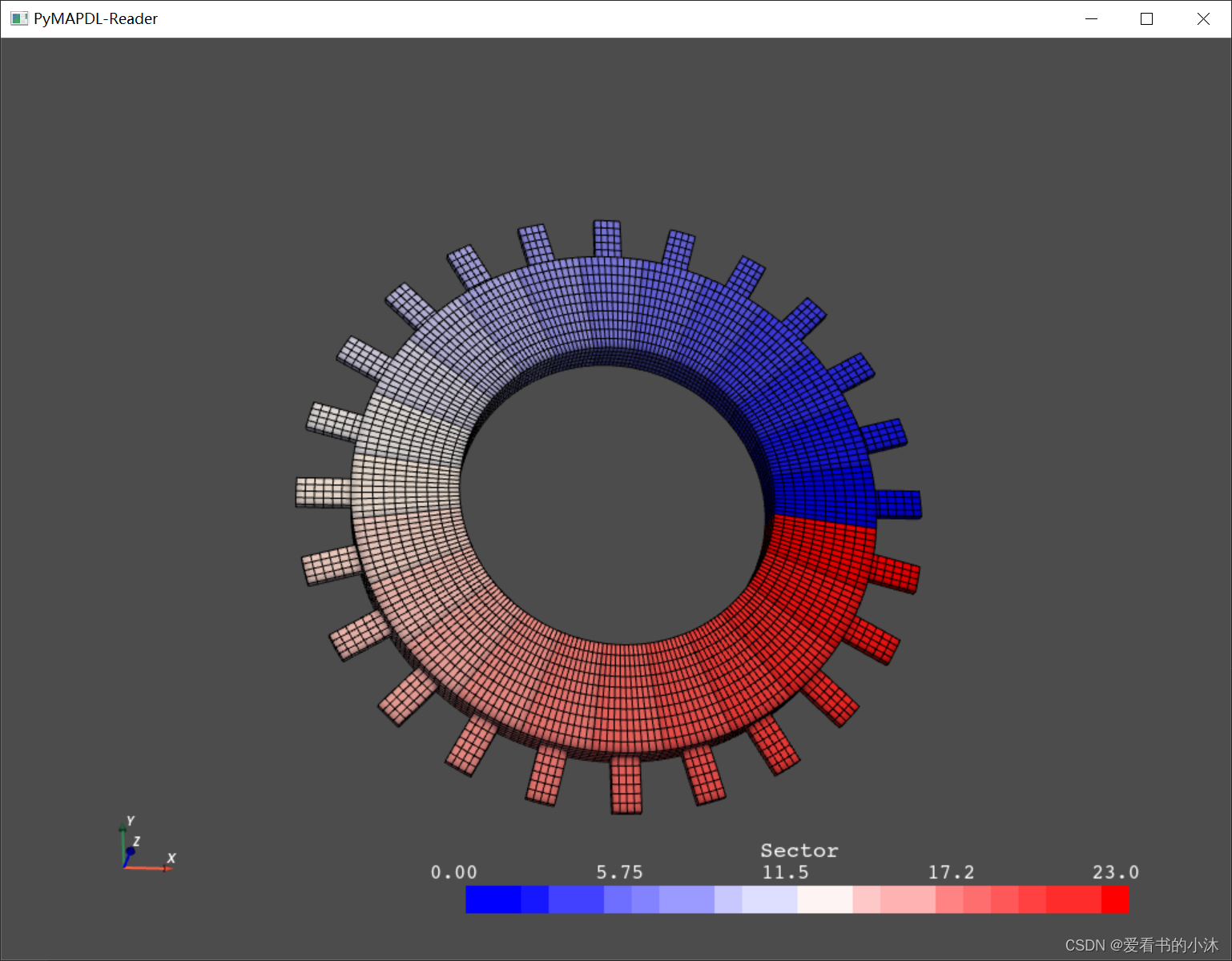
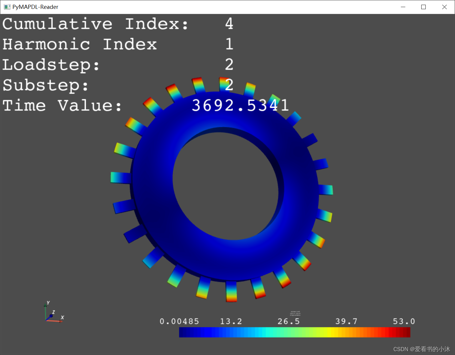
4.6 Understanding Nodal Diameters from a Cyclic Model Analysis
从循环模型分析中了解节点直径。
此示例说明如何从来自模态分析的单叶片扇区和多叶片扇区的 MAPDL 结果文件中解释循环分析中的模态。
import numpy as np

from ansys.mapdl.reader import examples

rotor = examples.download_academic_rotor_result()
print(rotor)

# _ = rotor.plot_sectors(cpos='xy', stitle='Sector', smooth_shading=True, cmap='bwr')

## 您可以使用 MAPDL 的基于 1 的索引(加载步骤,子步骤)来引用结果集。
# _ = rotor.plot_nodal_displacement((2, 2), comp='norm', cpos='xy')

## 您可以使用累积索引来参考结果。
# _ = rotor.plot_nodal_displacement(10, comp='norm', cpos='xy')

_ = rotor.animate_nodal_displacement((3, 1), displacement_factor=0.03,
                                     n_frames=30, show_axes=False, background='grey',
                                     loop=False, add_text=True,
                                     movie_filename='rotor1.gif')
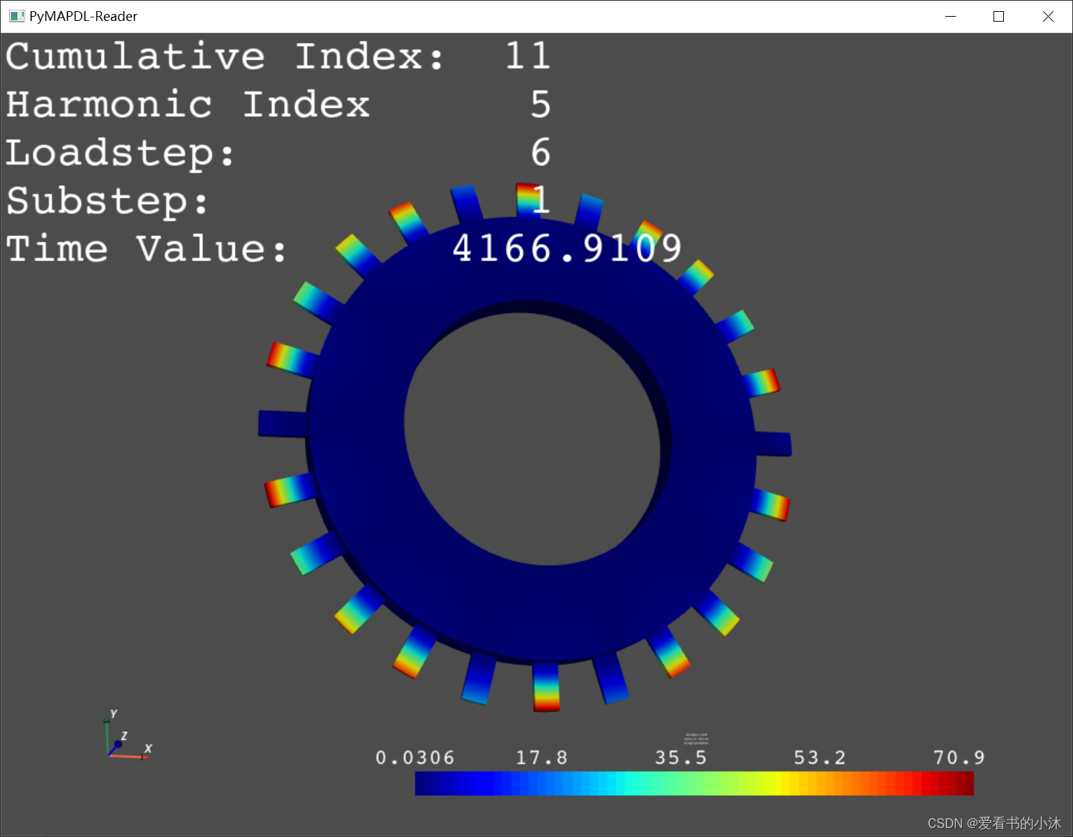
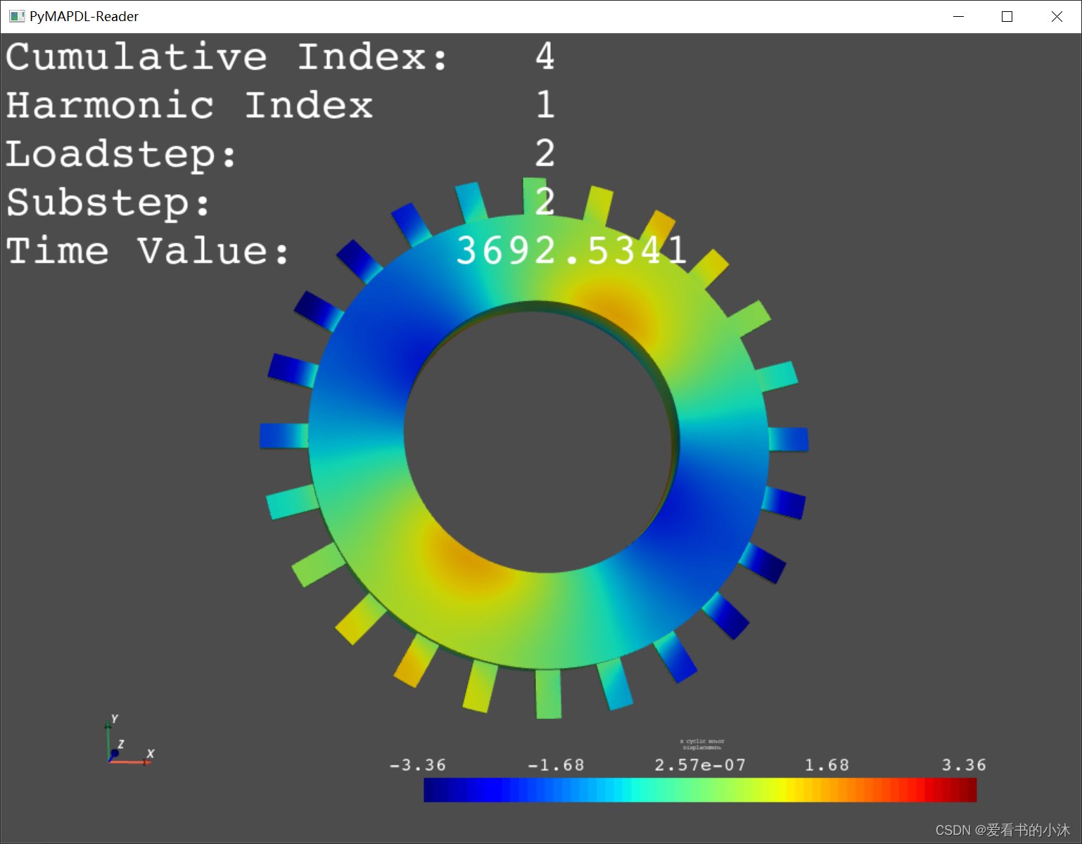
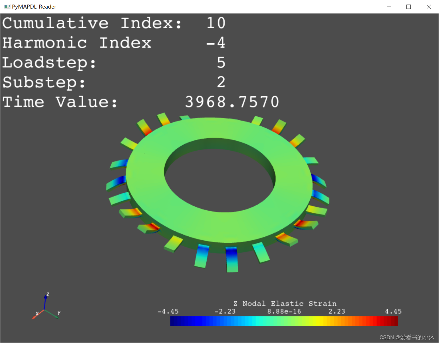
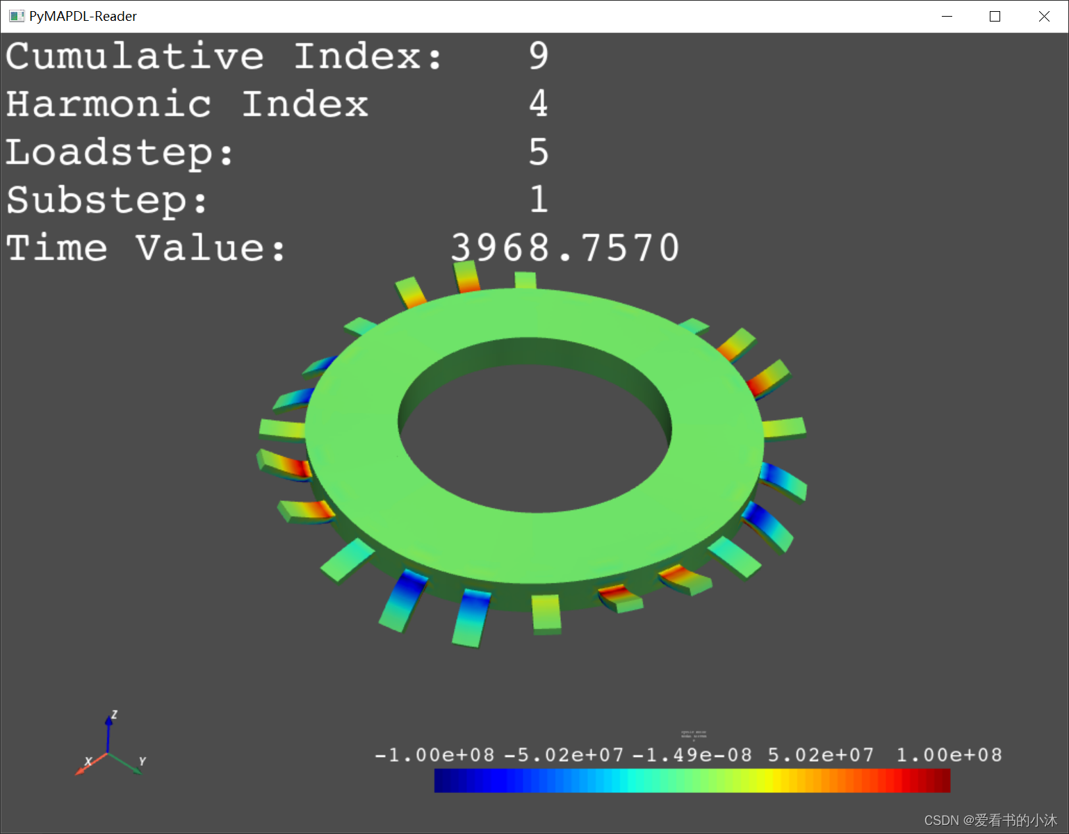
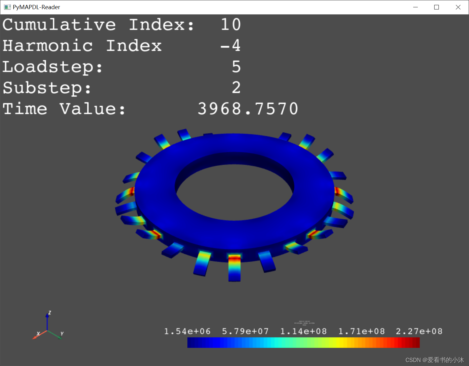
4.7 Stress and Strain from a Cyclic Modal Analysis(循环模态分析中的应力和应变)
循环模态分析中的应力和应变。
此示例说明如何从循环模态分析中提取应变和应力。
from ansys.mapdl.reader import examples

rotor = examples.download_academic_rotor_result()
print(rotor)

# _ = rotor.plot_nodal_displacement((2, 2), 'x', cpos='xy')

# nnum, strain = rotor.nodal_elastic_strain(3, full_rotor=True)

# _ = rotor.plot_nodal_elastic_strain((5, 2), 'Z', show_displacement=True,
#                                     displacement_factor=0.01)

# _ = rotor.plot_nodal_stress((5, 1), 'Z', show_displacement=True,
#                             displacement_factor=0.01)

#_ = rotor.plot_principal_nodal_stress((5, 2), 'SEQV', show_displacement=True,
#                                      displacement_factor=0.01)

_ = rotor.animate_nodal_displacement((2, 2), displacement_factor=0.03,
                                     n_frames=50, show_axes=False, background='grey',
                                     loop=False, add_text=True,
                                     movie_filename='rotor2.gif')
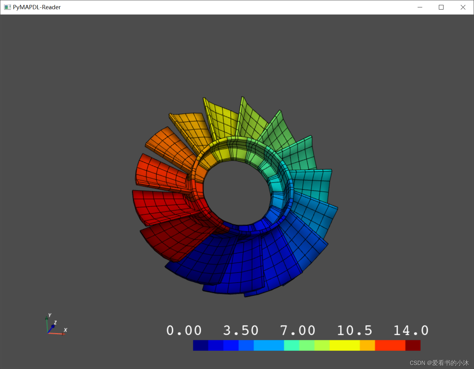
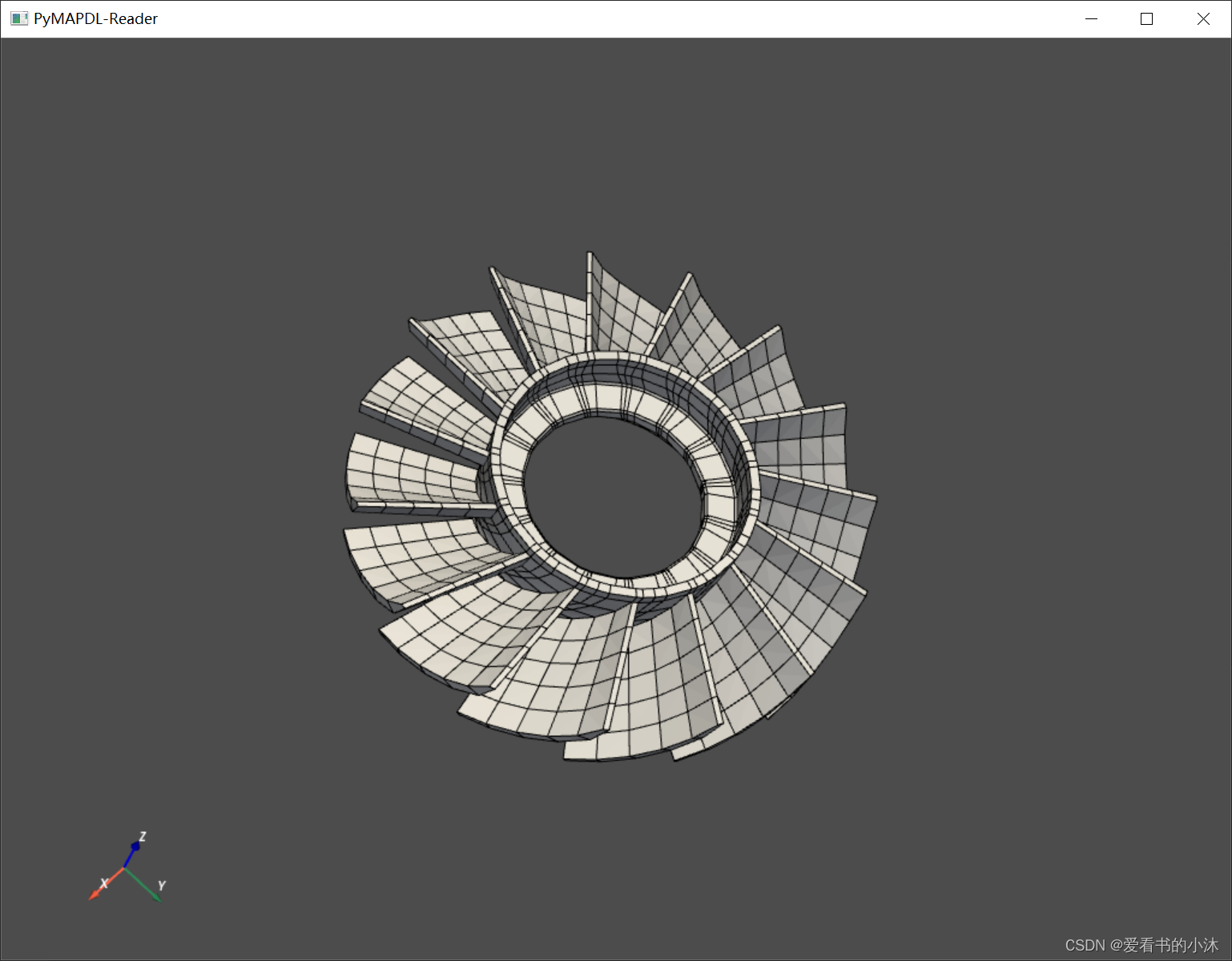
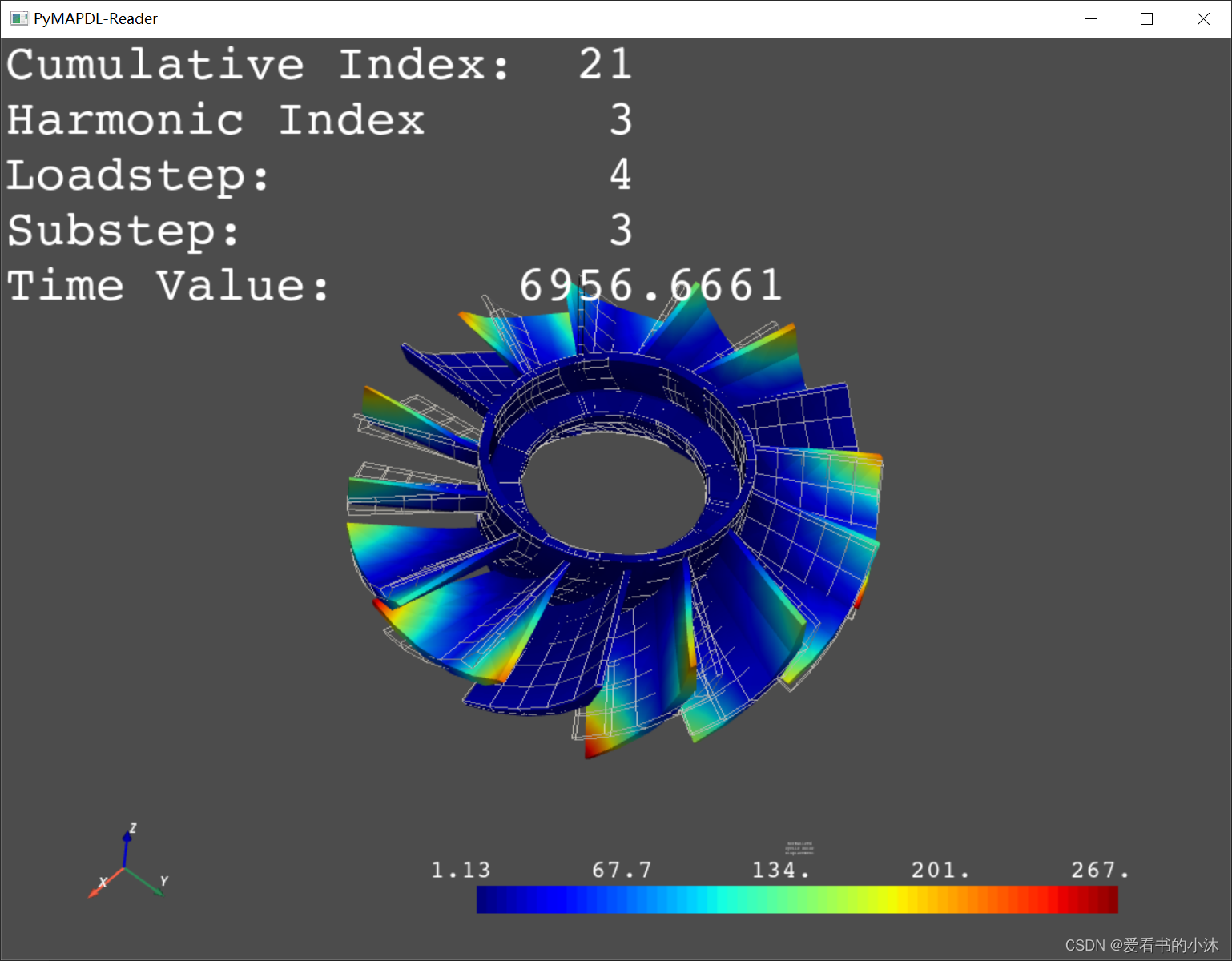
4.8 Cyclic Model Visualization(动画完整的循环模型)
可视化和动画完整的循环模型。该模型基于 jetcat 转子。
# sphinx_gallery_thumbnail_number = 2
from ansys.mapdl.reader import examples

rotor = examples.download_sector_modal()
print(rotor)

# rotor.plot_sectors(cpos='xy', smooth_shading=True)
# rotor.plot()

# rotor.plot_nodal_displacement(20, show_displacement=True,
#                               displacement_factor=0.001,
#                               overlay_wireframe=True)  # same as (2, 4)


rotor.animate_nodal_solution(20, loop=False, movie_filename='rotor_mode.gif',
                             background='w', displacement_factor=0.001,
                             add_text=False,
                             n_frames=30)
5、个人测试示例
5.1 加载rst结果文件
(1)Reads ANSYS-written binary files:
- Jobname.RST: Result file from structural analysis
- Jobname.RTH: Result file from a thermal analysis
- Jobname.EMAT: Stores data related to element matrices
- Jobname.FULL: Stores the full stiffness-mass matrix

(2)Examples
--------
>>> import pyansys
>>> result = pyansys.read_binary('file.rst')
>>> result = pyansys.read_binary('file.rst')
>>> full_file = pyansys.read_binary('file.full')
>>> emat_file = pyansys.read_binary('file.emat')
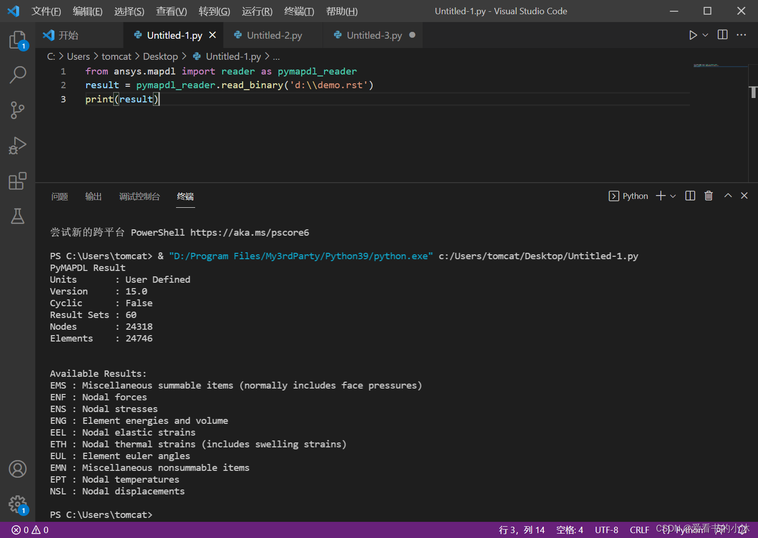
from ansys.mapdl import reader as pymapdl_reader
result = pymapdl_reader.read_binary('d:\\demo.rst')
print(result)
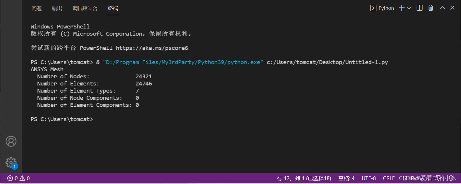
5.2 输出总体信息
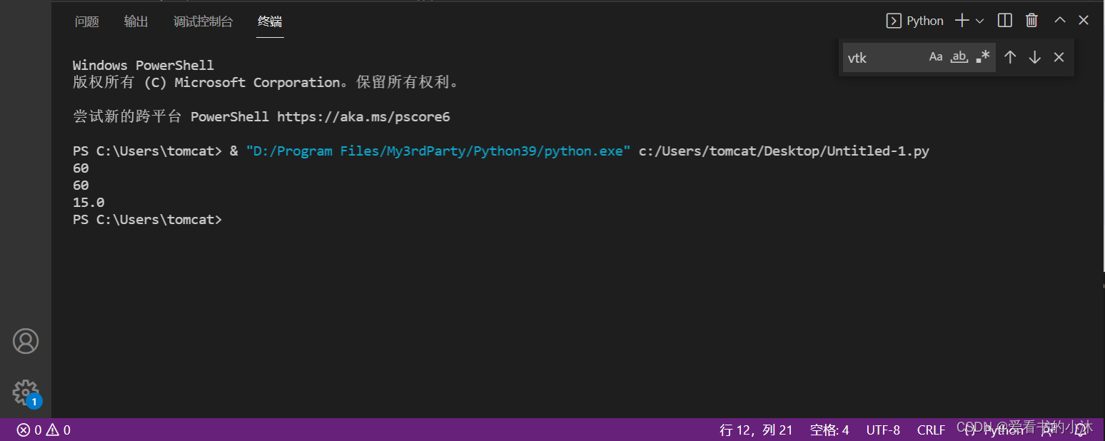
print(result.n_results)
print(result.nsets)
print(result.version)
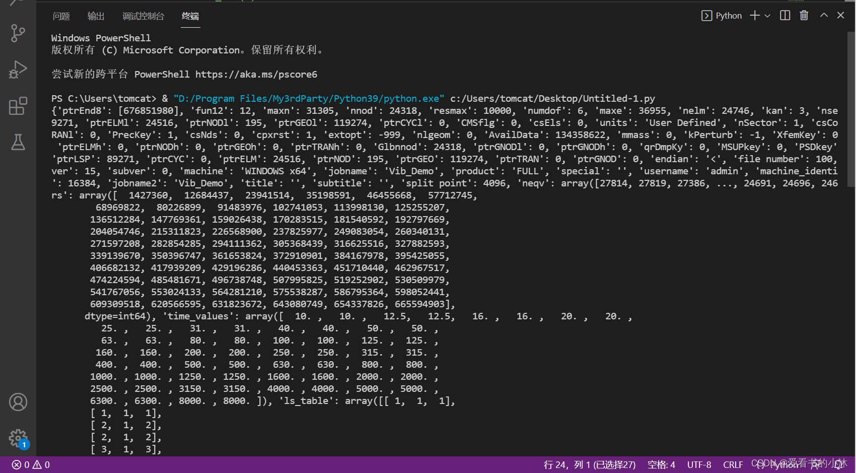
几何总体信息如下:
结果总体信息如下:
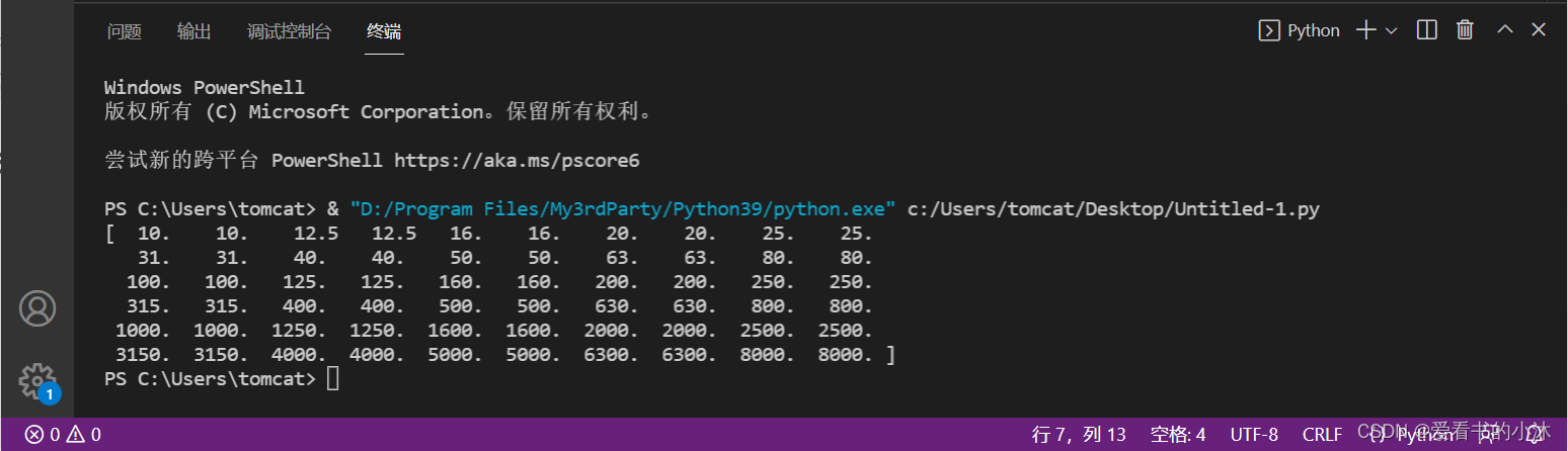
5.3 载荷频率数据以列表方式输出
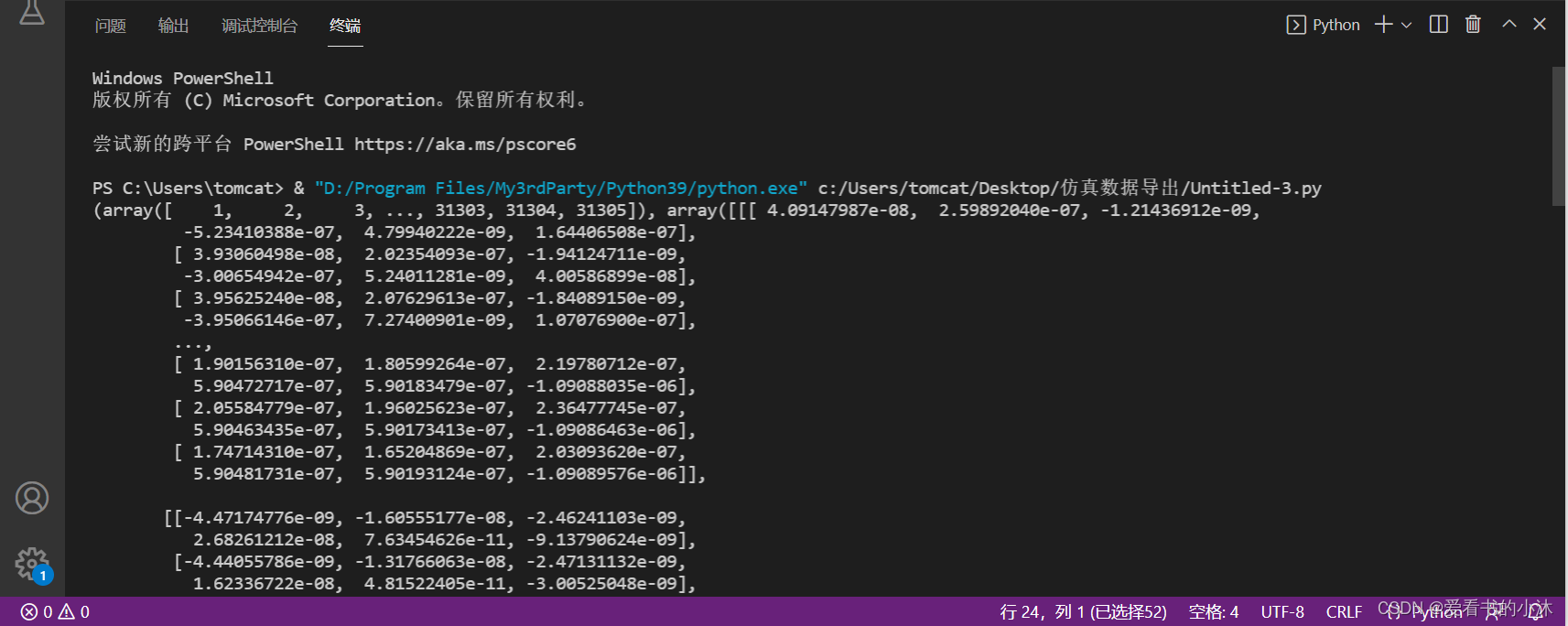
5.4 节点数据以列表方式输出
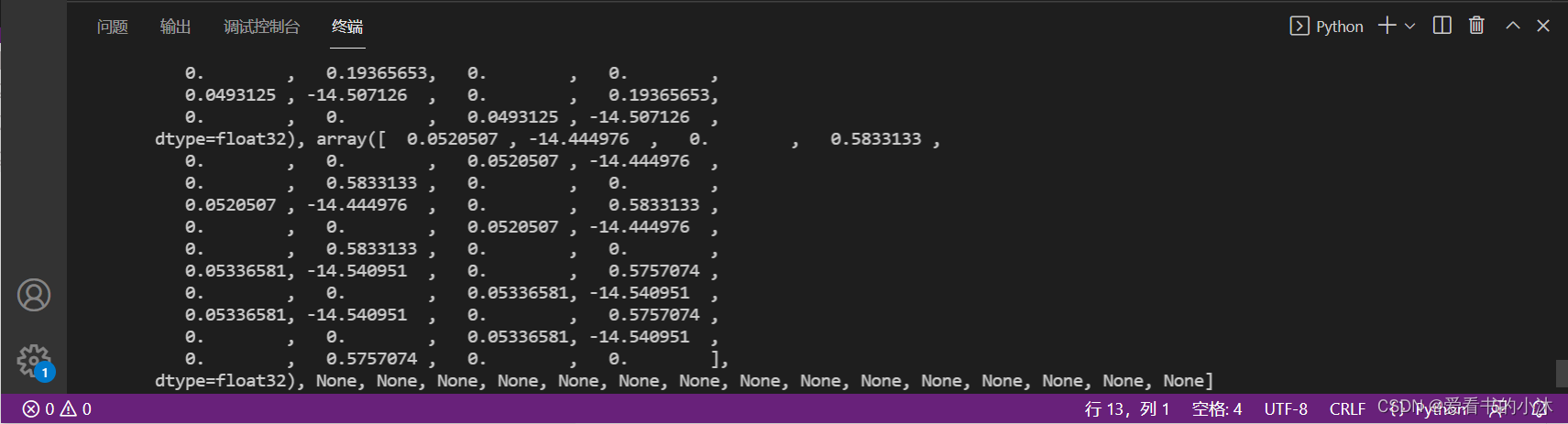
- 节点的结果位移和旋转信息输出
(3)方法3:
solution_type: str, optional
The solution type. Must be either nodal displacements('NSL'), nodal velocities ('VEL') or nodal
accelerations ('ACC').
# 节点的位移数据
data = result.nodal_time_history("NSL")
print(data)
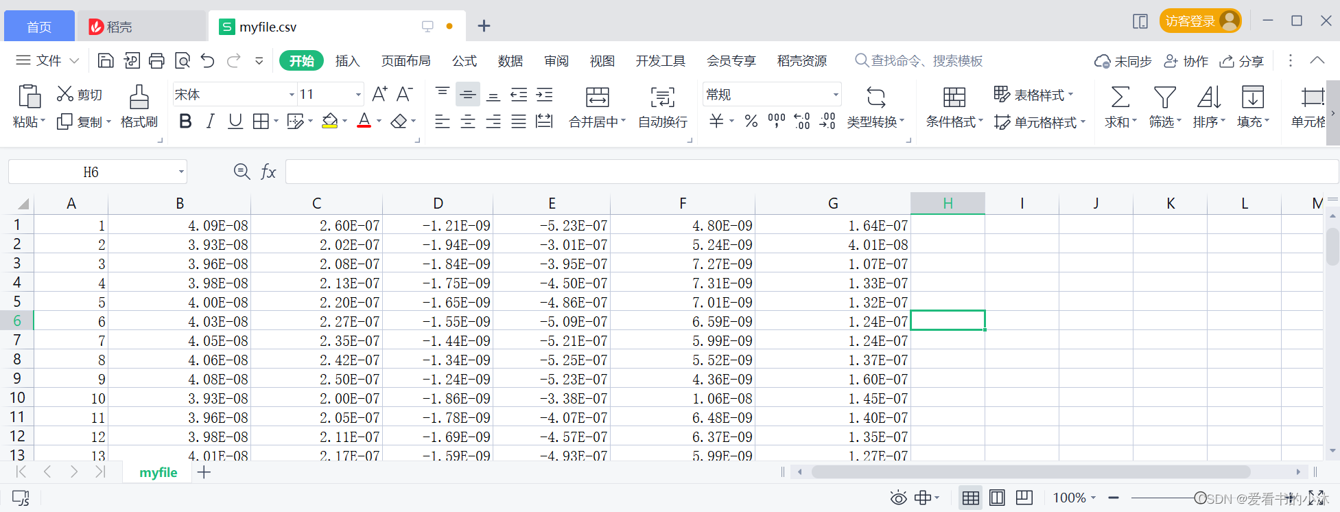
5.5 节点数据以文件方式输出
将结果数据存到本地CSV文件中:
import numpy as np

arr = np.column_stack((nnum, disp))
np.savetxt('d:\\myfile.csv', arr, delimiter=',')
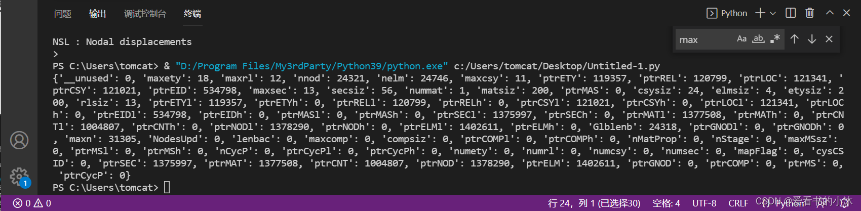
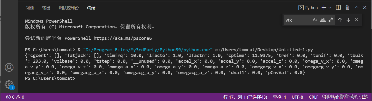
Return an informative dictionary of solution data for a result.
data = result.solution_info(0)
print(data)
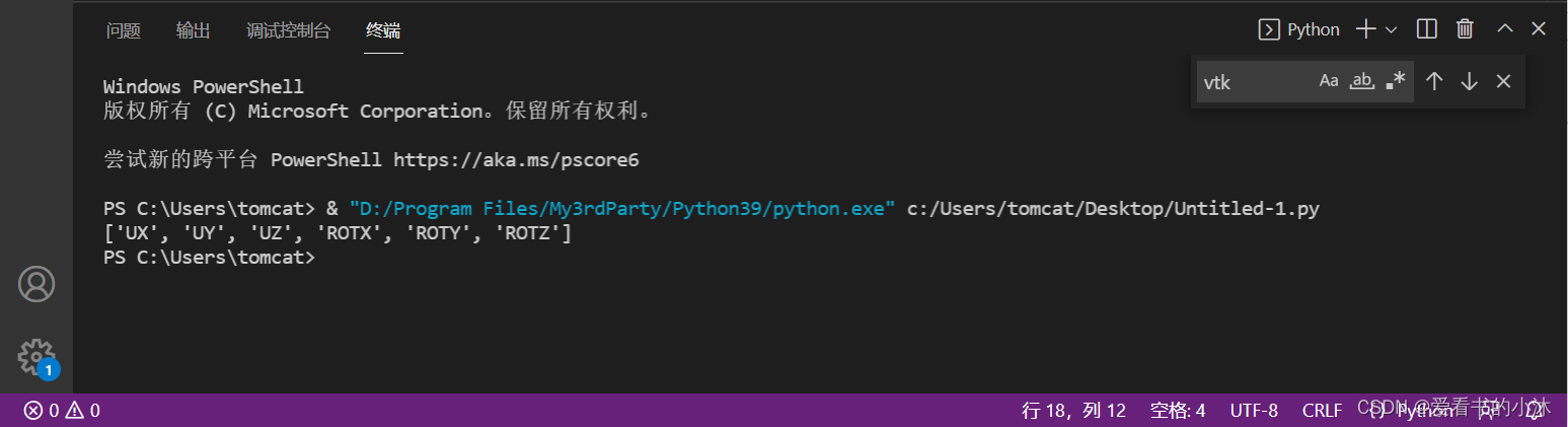
Return a list of degrees of freedom for a given result number.
data = result.result_dof(0)
print(data)
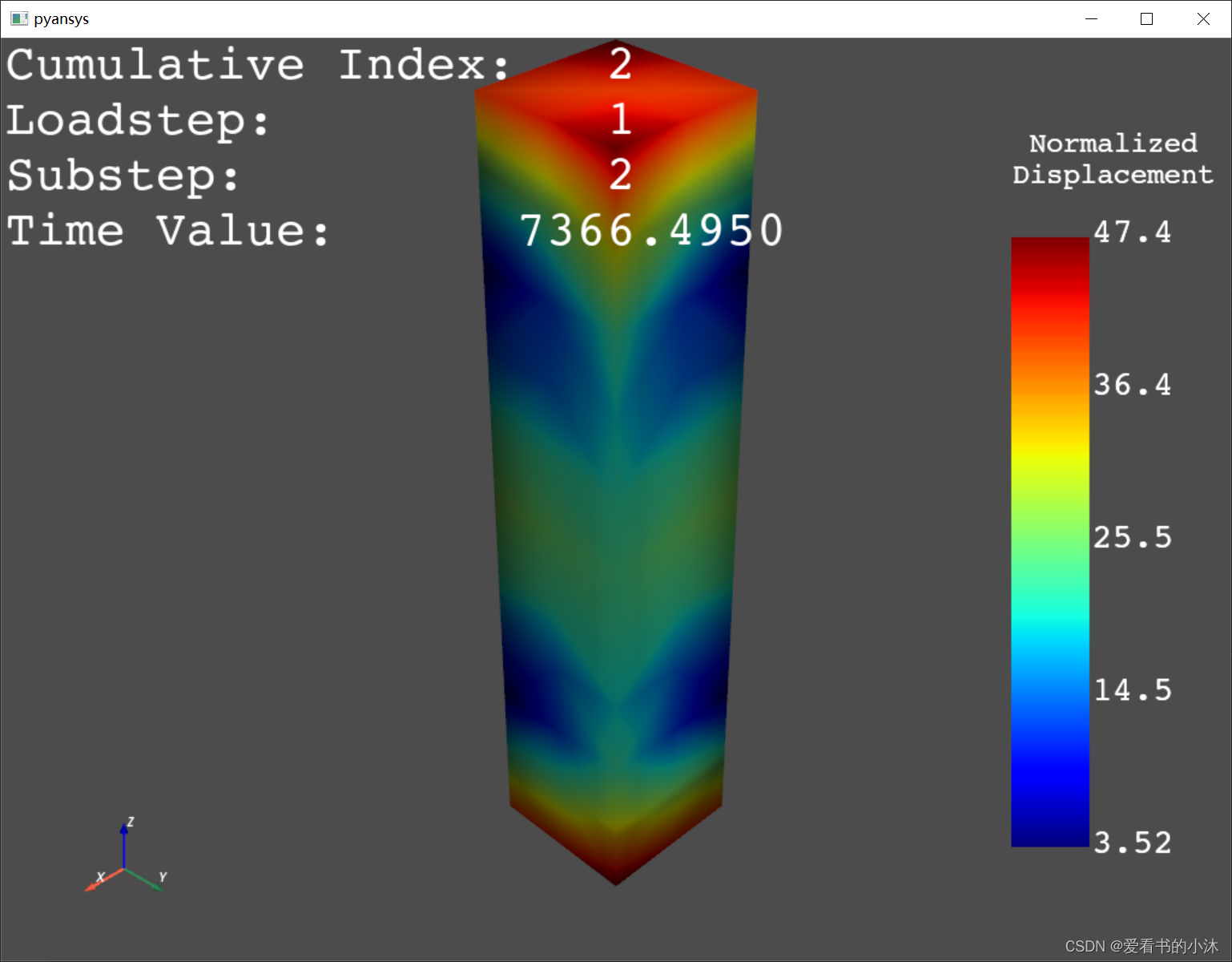
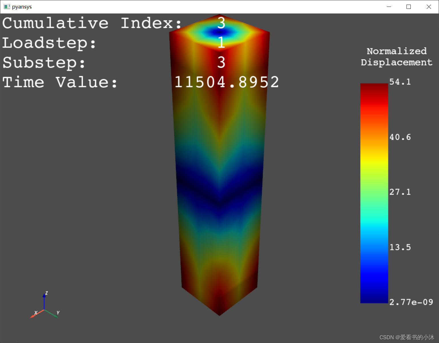
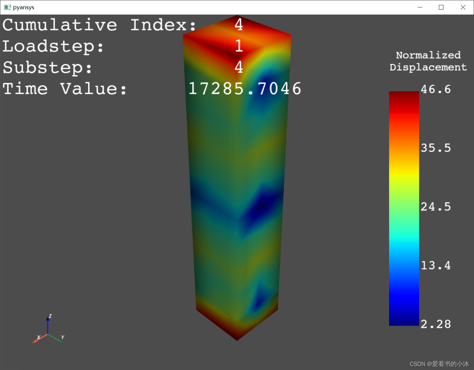
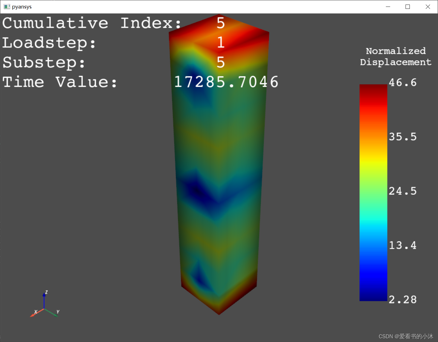
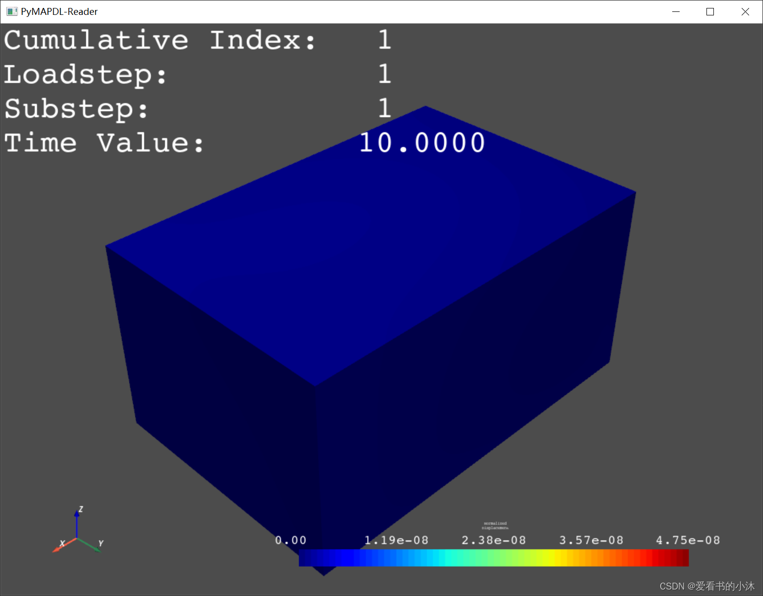
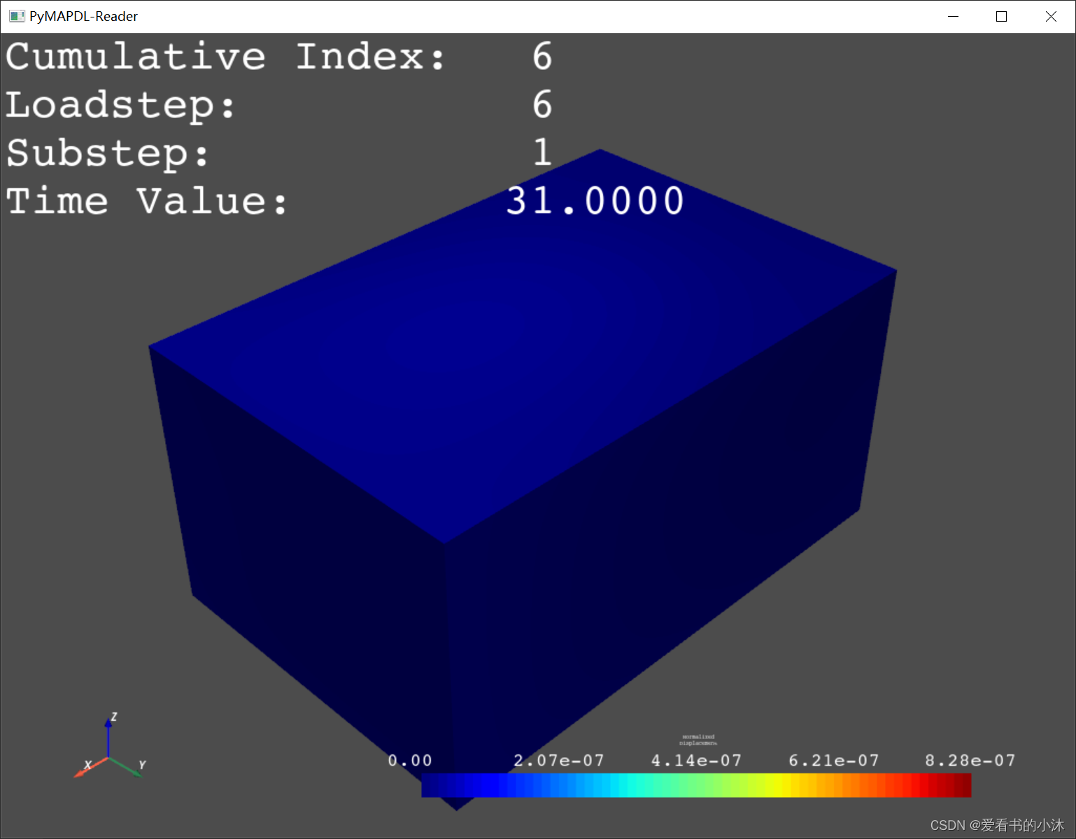
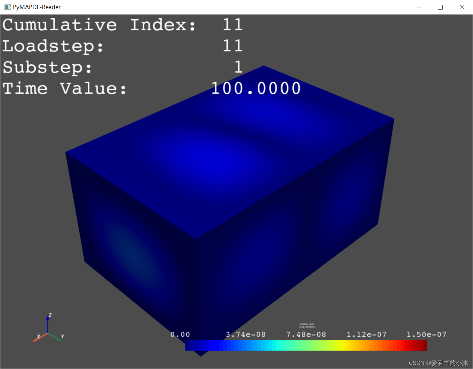
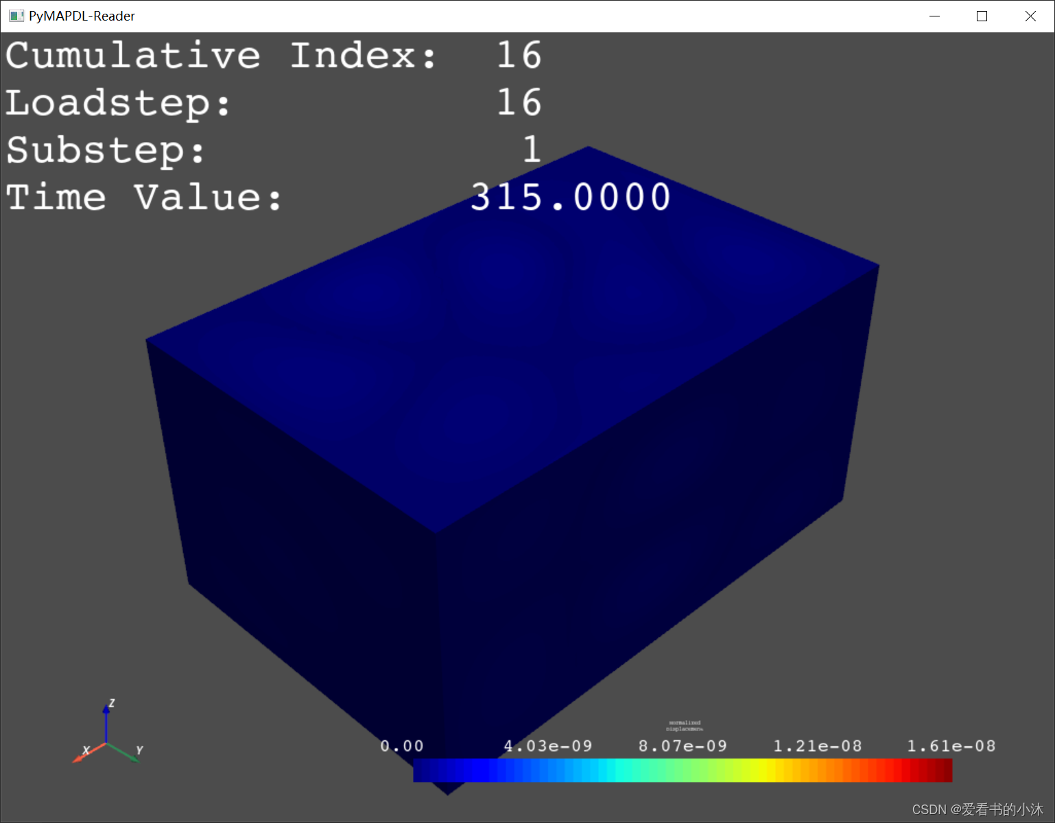
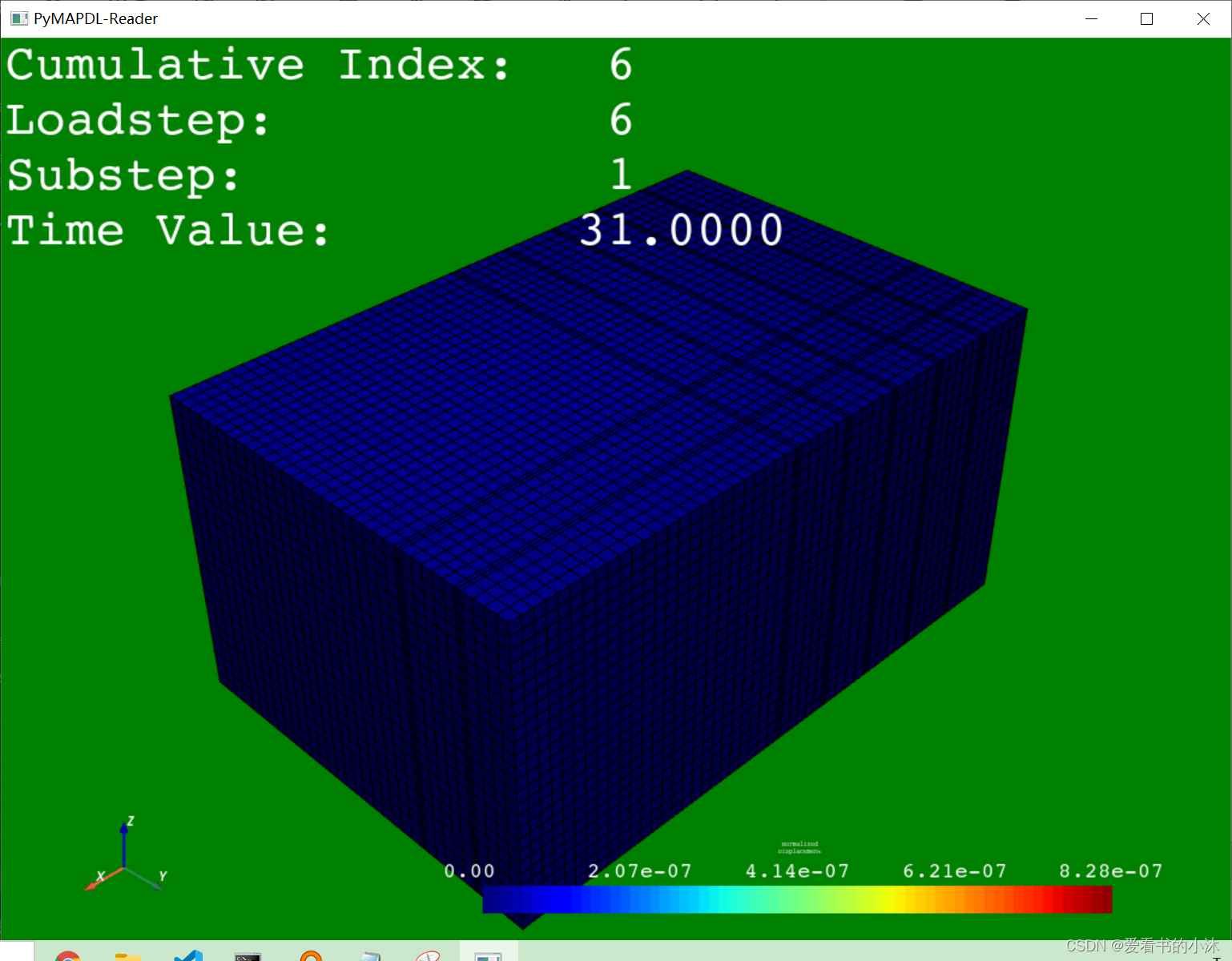
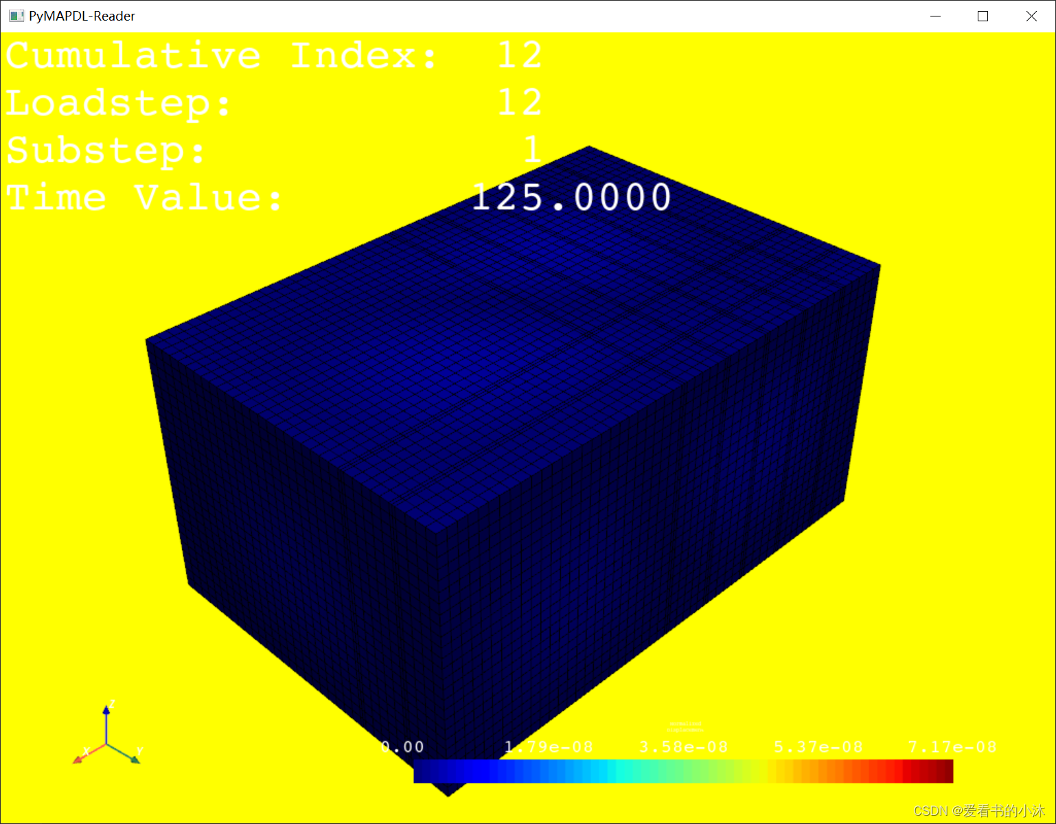
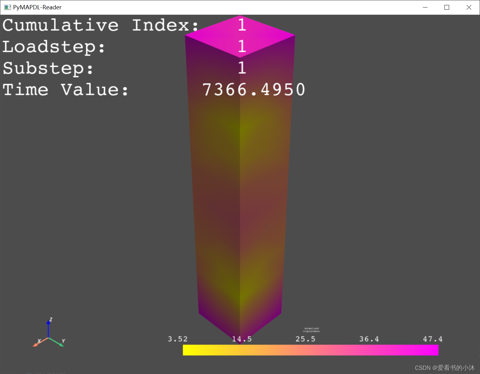
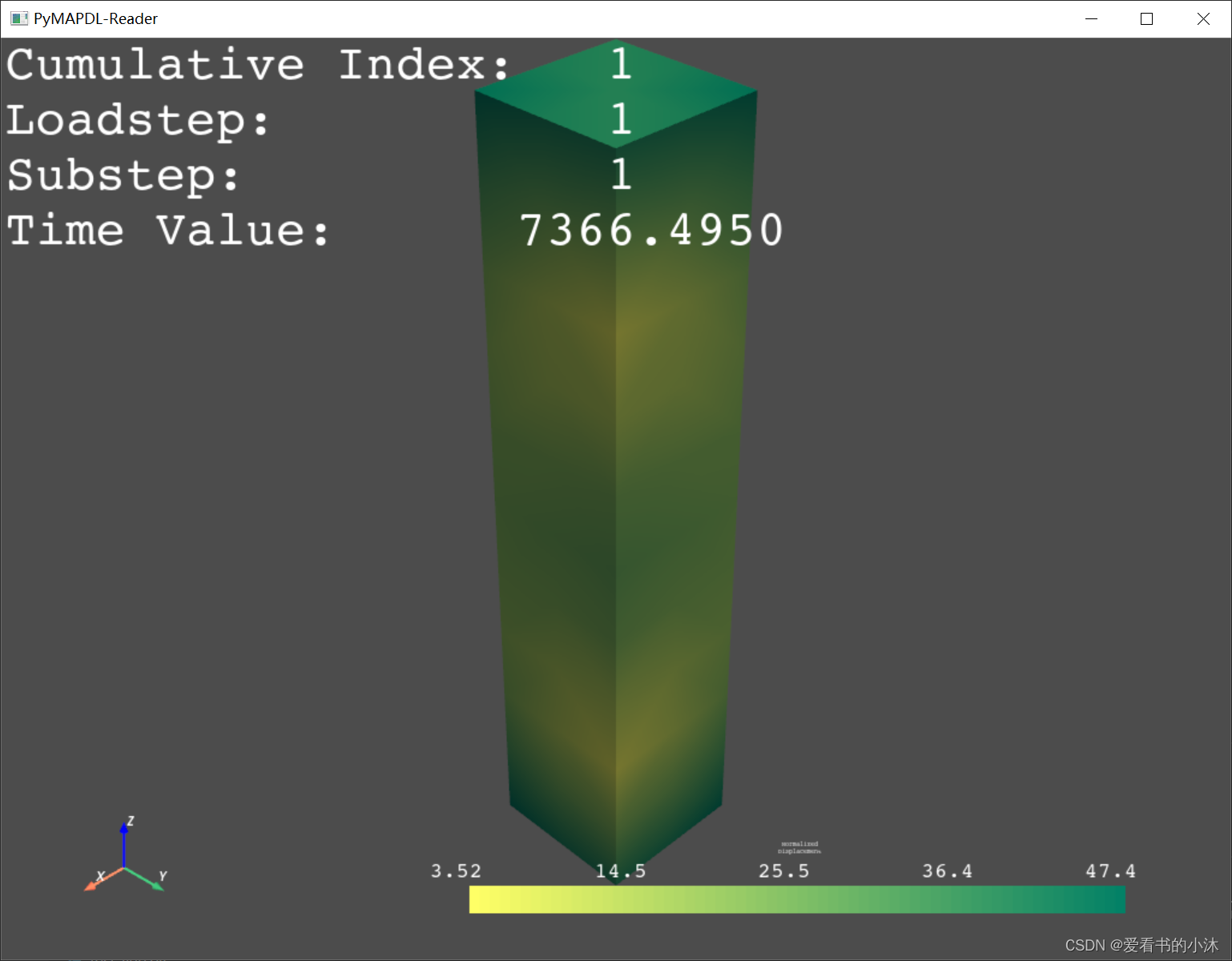
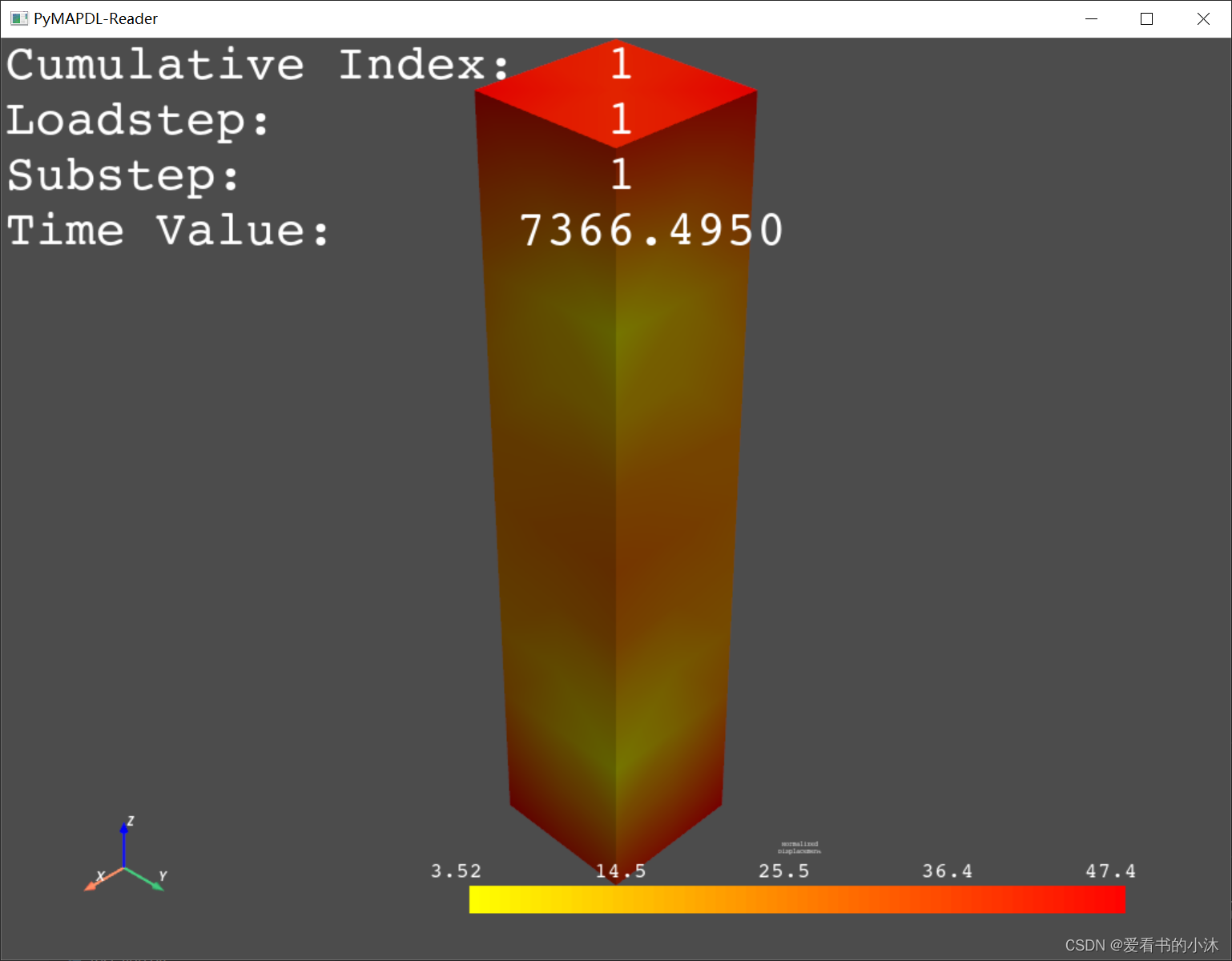
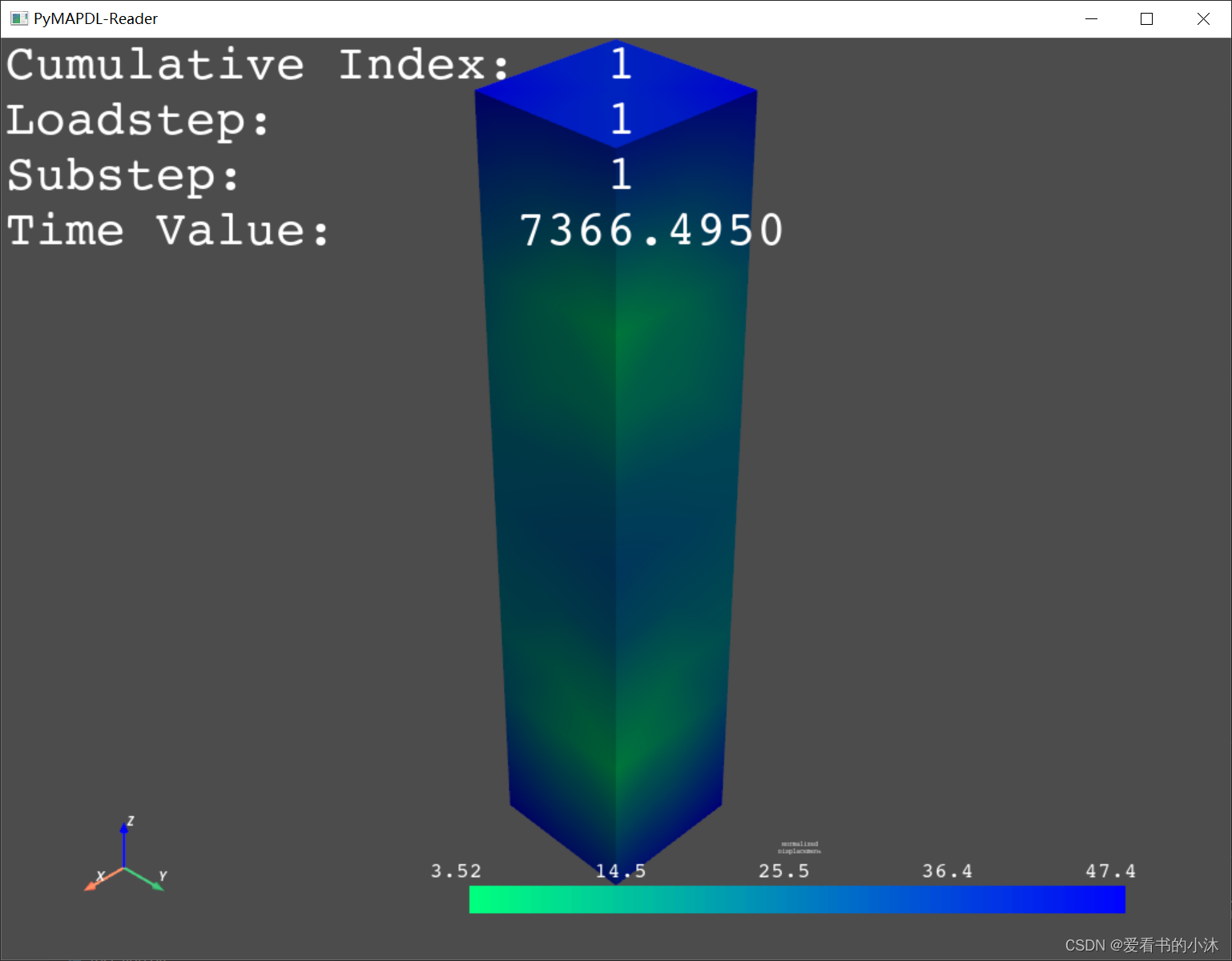
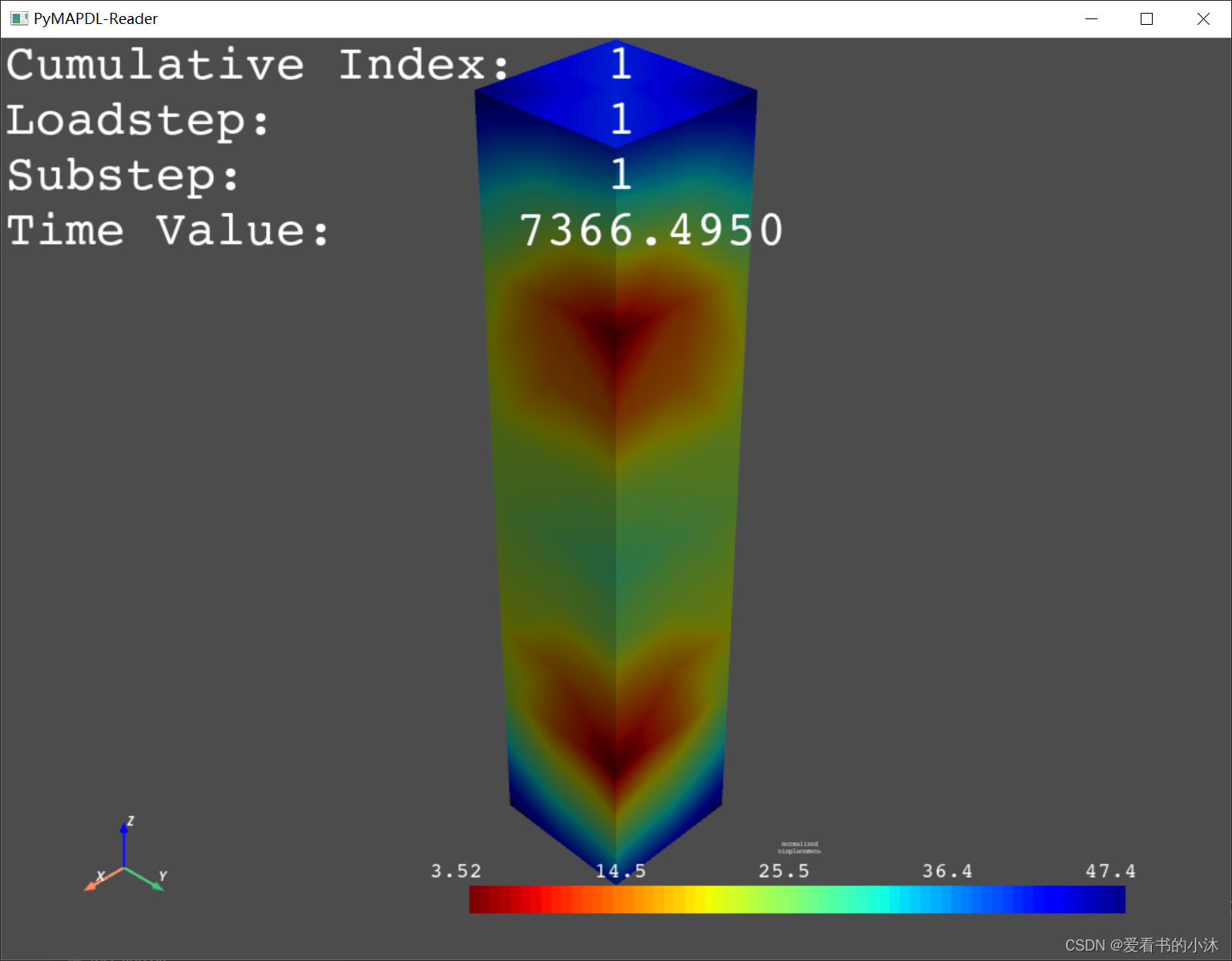
5.6 节点数据以绘图方式输出
Plots the nodal solution.
Defaults to “NORM” for a structural displacement result, and “TEMP” for a thermal result.
result.plot_nodal_solution(0)
result.plot_nodal_solution(10)
result.plot_nodal_solution(20)
result.plot_nodal_solution(30)
result.plot_nodal_solution(11, background='g', show_edges=True)
result.plot_nodal_solution(22, background='y', show_edges=True)
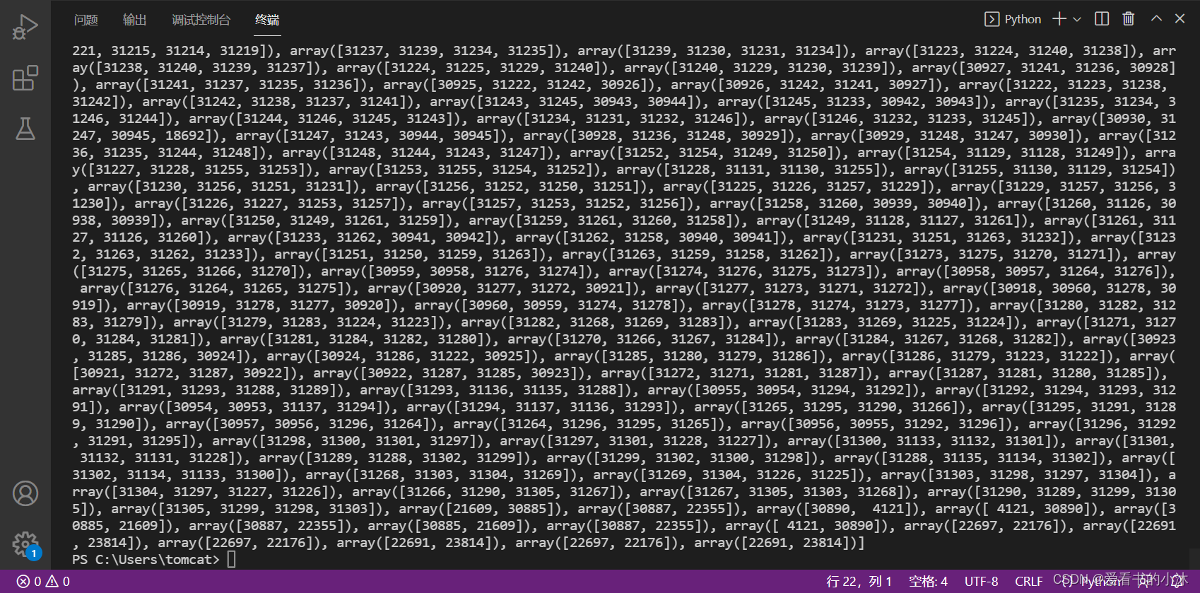
5.7 单元数据以列表方式输出
Element data type to retrieve:
        - EMS: misc. data
        - ENF: nodal forces
        - ENS: nodal stresses
        - ENG: volume and energies
        - EGR: nodal gradients
        - EEL: elastic strains
        - EPL: plastic strains
        - ECR: creep strains
        - ETH: thermal strains
        - EUL: euler angles
        - EFX: nodal fluxes
        - ELF: local forces
        - EMN: misc. non-sum values
        - ECD: element current densities
        - ENL: nodal nonlinear data
        - EHC: calculated heat generations
        - EPT: element temperatures
        - ESF: element surface stresses
        - EDI: diffusion strains
        - ETB: ETABLE items
        - ECT: contact data
        - EXY: integration point locations
        - EBA: back stresses
        - ESV: state variables
        - MNL: material nonlinear record
![[ 1 2 3 ... 36953 36954 36955]](https://img-blog.csdnimg.cn/e166c246890240fb902f0b85f3aad6e8.png?x-oss-process=image/watermark,type_d3F5LXplbmhlaQ,shadow_50,text_Q1NETiBA54ix55yL5Lmm55qE5bCP5rKQ,size_20,color_FFFFFF,t_70,g_se,x_16)
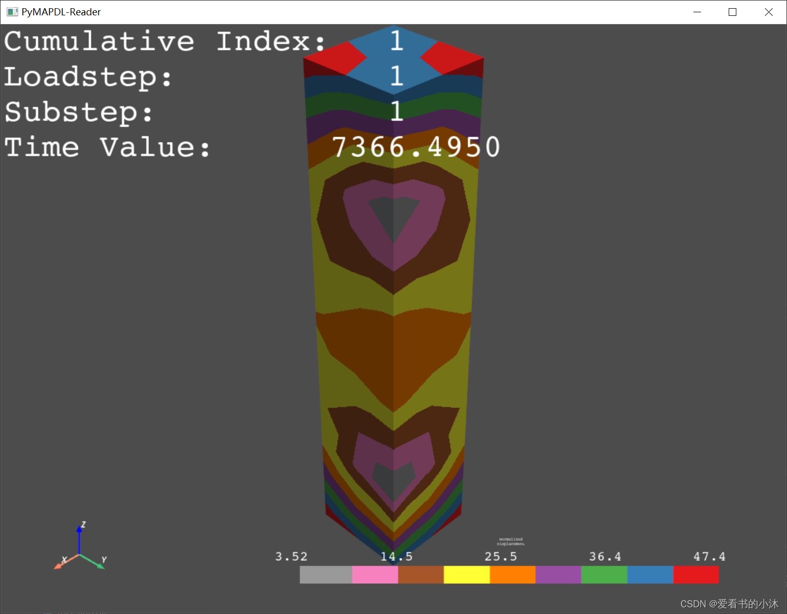
5.8 自定义plot绘图颜色表


结语
如果您觉得该方法或代码有一点点用处,可以给作者点个赞,或打赏杯咖啡;╮( ̄▽ ̄)╭
如果您感觉方法或代码不咋地//(ㄒoㄒ)//,就在评论处留言,作者继续改进;o_O???
如果您需要相关功能的代码定制化开发,可以留言私信作者;(✿◡‿◡)
感谢各位大佬童鞋们的支持!( ´ ▽´ )ノ ( ´ ▽´)っ!!!
文章出处登录后可见!