最近看到FBCSP的论文,但是不了解CSP是个啥,所以就学习了一下,这里记录一下,以下内容主要来自以下文章:共空间模式算法(CSP);特征提取丨共空间模式 Common Spatial Pattern (CSP);Python中MNE库利用CSP分析运动想象数据。
共空间模式算法(CSP)
共空间模式算法(Common Spatial Pattern,CSP)广泛应用于脑机接口(Brain-Computer Interface,BCI)中脑电信号(Electroencephalogram,EEG)的特征提取,因此,在介绍CSP算法前,有必要对脑电接口,脑电信号等相关概念做个简述。
1 BCI与EEG的基础概念
- BCI: 脑机接口(brain-computer interface, BCI),指在人或动物大脑与外部设备之间创建的直接连接,实现脑与设备的信息交换;
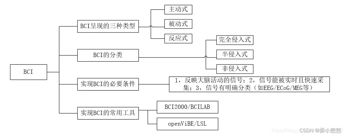
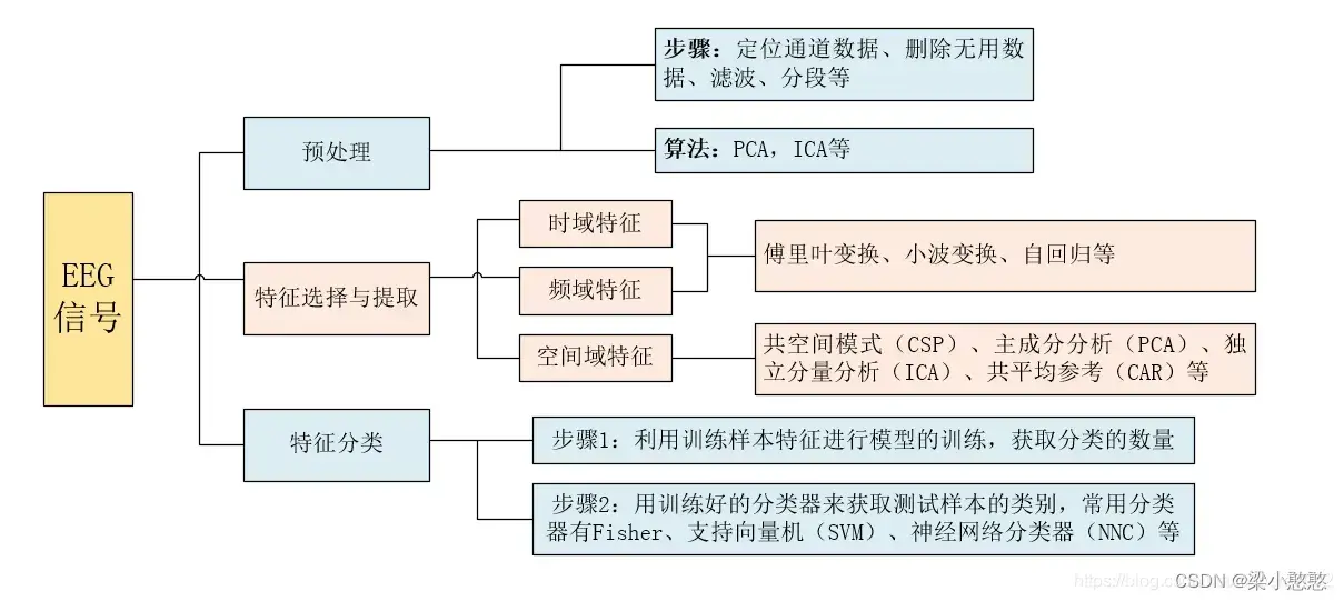
- EEG: 脑电信号(EEG)是一种 5-100μv和低频的生物电信号,需放大后才能显示和处理。在脑电信号处理与模式识别系统中,为了正确的识别 EEG 信号,信号的处理应该包括以下三个部分:预处理、特征选择与提取以及 特征分类。信号预处理主要为了去除低频噪声干扰,如利用空间滤波器(CAR)滤除眼电、肌电等低频噪声干扰。特征提取与选择主要是为了降低脑电数据的维数和提取出与分类相关的特征。
目前,EEG数据的特征主要有三种:时域特征、频域特征与空域特征,不同的特征需要采取不同的特征提取方法,如空域特征一般采用空域滤波器(共同空间模式,CSP)进行提取,频域特征一般采用傅立叶变换、小波变换或自回归(Auto-Regressive, AR)模型获取。特征分类主要是利用分类算法对提取到的特征进行分类,主要分为两个步骤:首先,利用训练样本特征进行模型的训练,获取分类的参数,然后,用训练好的分类器来获取测试样本特征的类别。目前,较常用的分类器有 Fisher、支持向量机(SVM)、神经网络分类器(Neural network classifier)和贝叶斯分类器(Bayesian classifier)等。
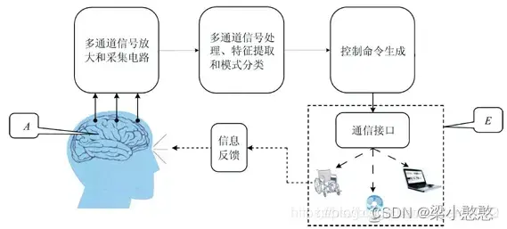
- EEG-BCI: 系统组成示意图如下:
2 CSP算法简介
2.1 储备知识
- 空间滤波器(spatial filters)
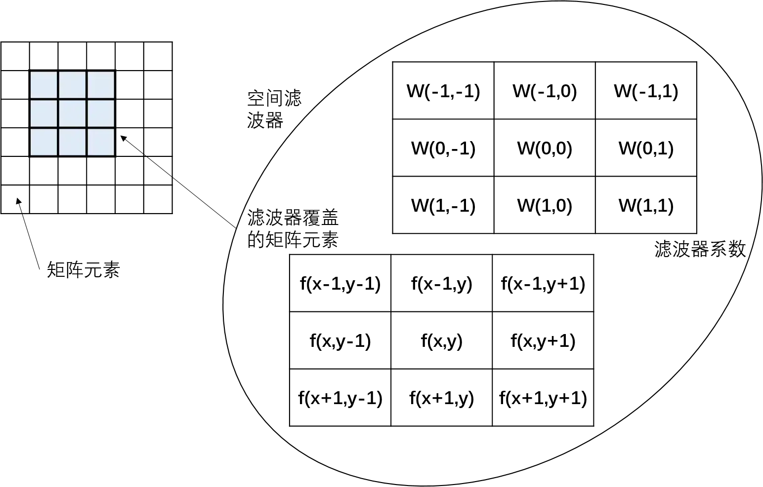
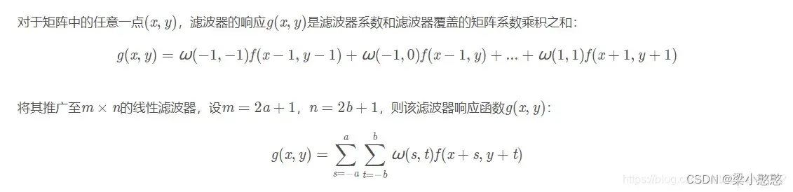
滤波是指通过操作接受或拒绝一定的频率。具体到空间滤波器,指的是通过空间滤波器对矩阵的元素进行修改,达到预期的效果。
空间滤波器由一下两部分组成:
1)一个邻域(通常为规模较小矩阵)
2)对该邻域的覆盖的矩阵元素执行的预定义操作
下图为使用3 × 3的邻域的线性空间滤波举例,过程就是对原矩阵的元素逐个按照预选定义的滤波器的操作进行运算:
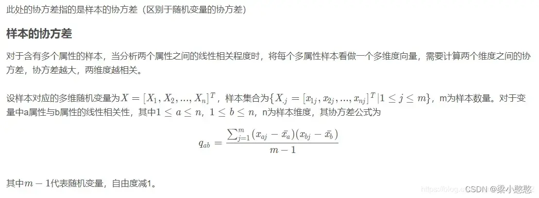
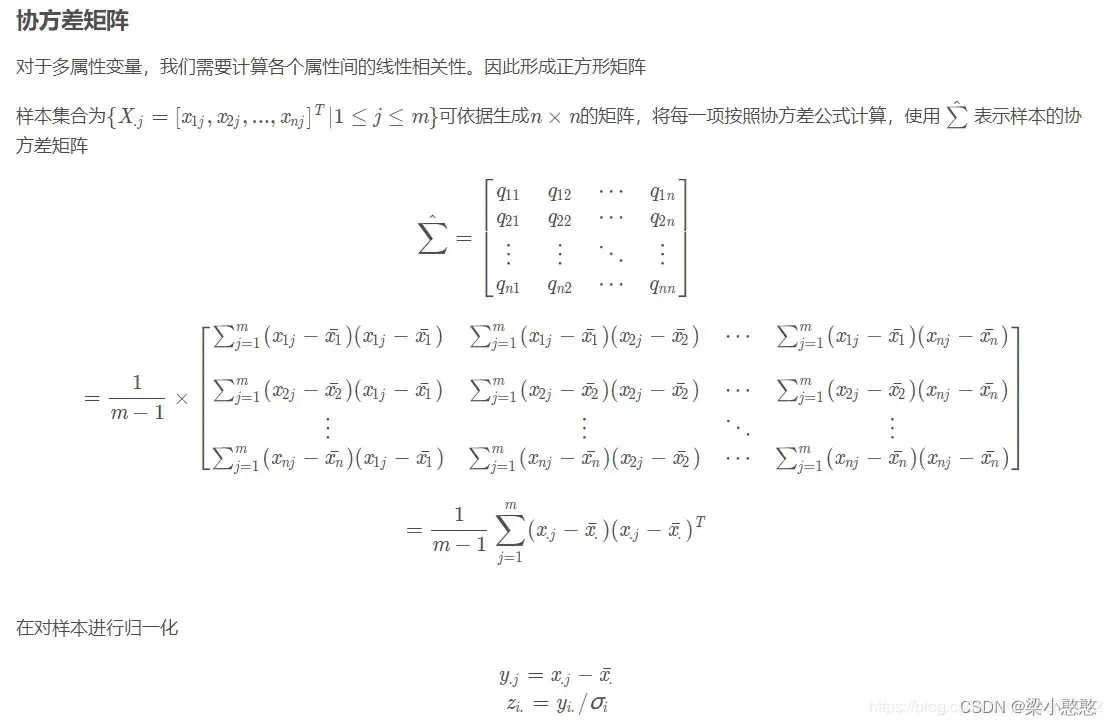
- 协方差与协方差矩阵
相关内容在这里也有介绍:【协方差】【相关系数】【协方差矩阵】【散度矩阵】

- 方阵特征值与特征向量

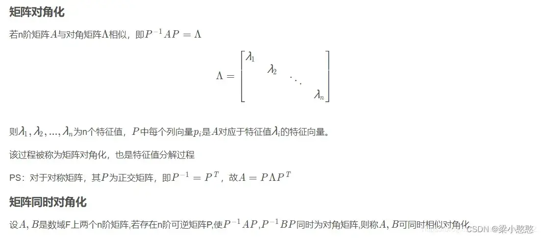
- 矩阵对角化及同时对角化
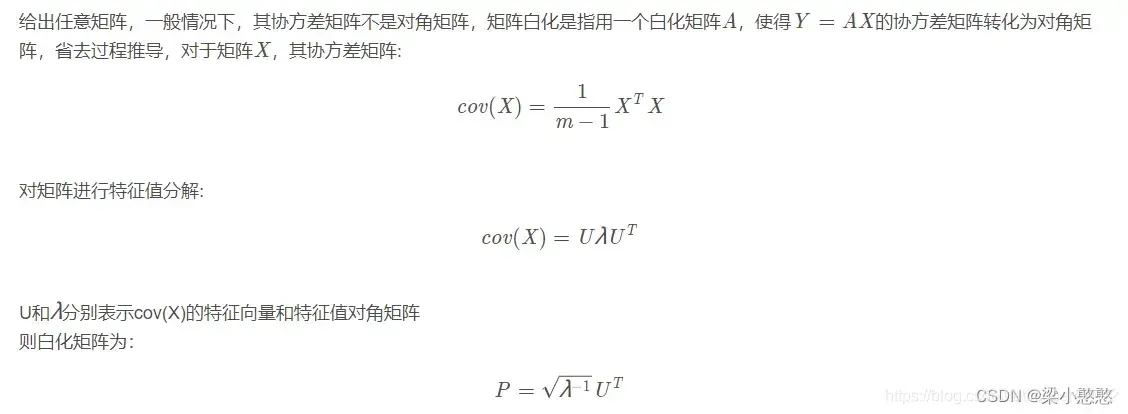
- 矩阵白化
相关内容在这里也有介绍:矩阵白化原理及推导
2.2 基本概念
共空间模式(CSP): 一种对两分类任务下的空域滤波特征提取算法,能够从多通道的脑机接口数据里面提取出每一类的空间分布成分。
共空间模式算法的基本原理: 利用矩阵的对角化,找到一组最优空间滤波器进行投影,使得两类信号的方差值差异最大化,从而得到具有较高区分度的特征向量。
共空间模式算法旨在: 设计空间滤波器使得两组脑电时空信号矩阵滤波后,方差值差异最大化,从而得到具有较高区分度的特征向量。用于下一步将特征向量送入分类器进行分类。
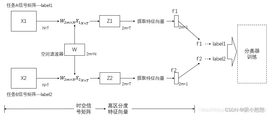
上图中,脑电时空信号矩阵的维数 ,
代表脑电通道数(导联数目),
代表时间层面的采样点个数。一个矩阵的单位为一个trail,表示一次测试。滤波器的维数是
,N同样代表导联数目,
为生成该滤波器时,人为设定的特征选取个数。
2.3 理论介绍
假设和
分别为两分类想象运动任务下的多通道诱发响应时-空信号矩阵,他们的维数均为
,
为脑电通道数,
为每个通道所采集的样本数。为了计算其协方差矩阵,现在假设
。在两种脑电想象任务情况下,一般采用复合源的数学模型来描述
信号,为了方便计算,一般忽略噪声所产生的影响。
和
可以分别写成:

式中:和
分别代表两种类型任务。不妨假设这两个源信号是相互线性独立的;
代表两种类型任务下所共同拥有的源信号,假设
是由
个源所构成的,
是由
个源所构成。
则和
便是由
和
相关的
和
个共同空间模式组成的,由于每个空间模式都是一个
维的向量,现在用这个向量来表示单个的源信号所引起的信号在
个导联上的分布权重。
表示的是与
相应的共有的空间模式。
算法的目标就是要设计空间滤波器
和
得到空间因子
。
2.3.1 求2类数据的混合空间协方差矩阵
和
归一化后的协方差矩阵
和
分别为:

2.3.2 应用主成分分析法,求出白化特征值矩阵P
对混合空间协方差矩阵按式进行特征值分解:

则有,此结论由白化矩阵得到。
2.3.3 构造空间滤波器
对和
进行如下变换:
然后对和
做主分量分解,得到:
其中和
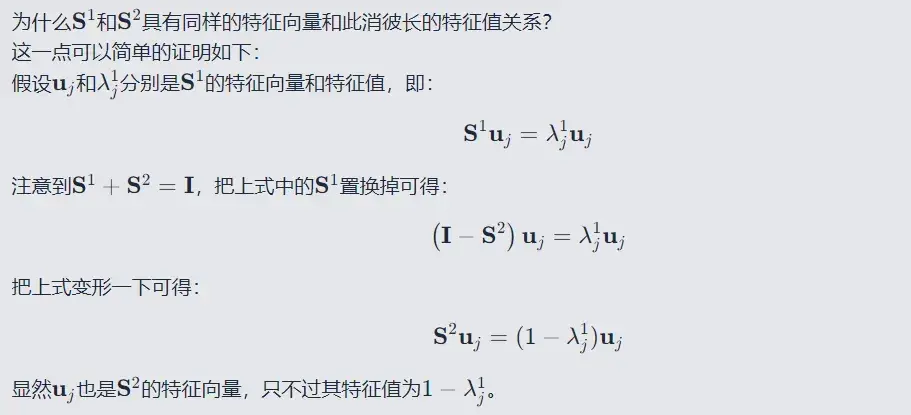
具有相同的特征向量(这也是共空间模式名称的由来):
这里假设的每一列是按照
中的特征值从大到小排列的,可以看出
中的特征值是从小到大排列的,满足
的关系。
把中的特征值按照降序排列,则
中对应的特征值按升序排列,根据这点可以推断出
和
具有下面的形式:
![]()
2.3.4 特征提取
将训练集的运动想象矩阵 经过构造的相应滤波器
滤波可得特征
为:
根据 CSP 算法在多电极采集脑电信号特征提取的定义,本研究选取 和
为想象左和想象右的特征向量,定义如下:


求出测试的 特征,进行下面的分类。
3 MATLAB 实现
3.1 构造空间滤波器
function CSPMatrix = learnCSP(EEGSignals,classLabels)
%
%Input:
%EEGSignals: the training EEG signals, composed of 2 classes. These signals
%are a structure such that:
%   EEGSignals.x: the EEG signals as a [Ns * Nc * Nt] Matrix where
%       Ns: number of EEG samples per trial
%       Nc: number of channels (EEG electrodes)
%       nT: number of trials
%   EEGSignals.y: a [1 * Nt] vector containing the class labels for each trial
%   EEGSignals.s: the sampling frequency (in Hz)
%
%Output:
%CSPMatrix: the learnt CSP filters (a [Nc*Nc] matrix with the filters as rows)
%
%See also: extractCSPFeatures

%check and initializations
nbChannels = size(EEGSignals.x,2);
nbTrials = size(EEGSignals.x,3);
nbClasses = length(classLabels);

if nbClasses ~= 2
    disp('ERROR! CSP can only be used for two classes');
    return;
end

covMatrices = cell(nbClasses,1); %the covariance matrices for each class

% Computing the normalized covariance matrices for each trial
trialCov = zeros(nbChannels,nbChannels,nbTrials);
for t=1:nbTrials
    E = EEGSignals.x(:,:,t)';                       %note the transpose
    EE = E * E'; % 计算单试次的协方差矩阵
    trialCov(:,:,t) = EE ./ trace(EE);
end
clear E;
clear EE;

%computing the covariance matrix for each class
for c=1:nbClasses
    covMatrices{c} = mean(trialCov(:,:,EEGSignals.y == classLabels(c)),3); %EEGSignals.y==classLabels(c) returns the indeces corresponding to the class labels
end

%the total covariance matrix
covTotal = covMatrices{1} + covMatrices{2};


%whitening transform of total covariance matrix
[Ut Dt] = eig(covTotal); %caution: the eigenvalues are initially in increasing order
eigenvalues = diag(Dt);
[eigenvalues egIndex] = sort(eigenvalues, 'descend');
Ut = Ut(:,egIndex);
P = diag(sqrt(1./eigenvalues)) * Ut'; % 白化变换矩阵

%transforming covariance matrix of first class using P
transformedCov1 =  P * covMatrices{1} * P';

%EVD of the transformed covariance matrix
[U1 D1] = eig(transformedCov1);
eigenvalues = diag(D1);
[eigenvalues egIndex] = sort(eigenvalues, 'descend');
U1 = U1(:, egIndex);
CSPMatrix = U1' * P; % 计算空间滤波器
3.2 特征提取
function features = extractCSP(EEGSignals, CSPMatrix, nbFilterPairs)
%
%extract features from an EEG data set using the Common Spatial Patterns (CSP) algorithm
%
%Input:
%EEGSignals: the EEGSignals from which extracting the CSP features. These signals
%are a structure such that:
%   EEGSignals.x: the EEG signals as a [Ns * Nc * Nt] Matrix where
%       Ns: number of EEG samples per trial
%       Nc: number of channels (EEG electrodes)
%       nT: number of trials
%   EEGSignals.y: a [1 * Nt] vector containing the class labels for each trial
%   EEGSignals.s: the sampling frequency (in Hz)
%CSPMatrix: the CSP projection matrix, learnt previously (see function learnCSP)
%nbFilterPairs: number of pairs of CSP filters to be used. The number of
%   features extracted will be twice the value of this parameter. The
%   filters selected are the one corresponding to the lowest and highest
%   eigenvalues
%
%Output:
%features: the features extracted from this EEG data set
%   as a [Nt * (nbFilterPairs*2 + 1)] matrix, with the class labels as the
%   last column
%
%initializations

nbTrials = size(EEGSignals.x,3);
features = zeros(nbTrials, 2*nbFilterPairs+1);
Filter = CSPMatrix([1:nbFilterPairs, (end-nbFilterPairs+1):end],:); % 取了CSPMatrix的前nbFilterPairs行和后nbFilterPairs行

%extracting the CSP features from each trial
for t=1:nbTrials
    %projecting the data onto the CSP filters
    %对通道做空间滤波,得到通道之间的空间关系,这个关系用几维矩阵表示,取决于滤波器的个数
    projectedTrial = Filter * EEGSignals.x(:,:,t)'; % [2*F, Ns] = [2*F,Nc] * [Nc, Ns]

    %generating the features as the log variance of the projected signals
    variances = var(projectedTrial,0,2); % [2*F, 1]
    for f=1:length(variances)
        features(t,f) = log(1+variances(f)); % 对协方差数值做了处理
    end
end
3.3 特征显示
% Extract Common Spatial Pattern (CSP) Feature
close all; clear; clc;
load dataset_BCIcomp1.mat
EEGSignals.x=x_train;
EEGSignals.y=y_train;
Y=y_train;
classLabels = unique(EEGSignals.y);
CSPMatrix = learnCSP(EEGSignals,classLabels);
nbFilterPairs = 1;
X = extractCSP(EEGSignals, CSPMatrix, nbFilterPairs);
EEGSignals.x=x_test;
T = extractCSP(EEGSignals, CSPMatrix, nbFilterPairs);
save dataCSP.mat X Y T
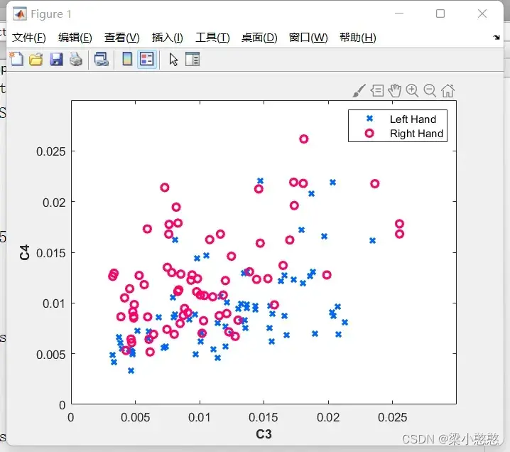
color_L = [0 102 255] ./ 255;
color_R = [255, 0, 102] ./ 255;
pos = find(Y==1);
plot(X(pos,1),X(pos,2),'x','Color',color_L,'LineWidth',2);
hold on
pos = find(Y==2);
plot(X(pos,1),X(pos,2),'o','Color',color_R,'LineWidth',2);
legend('Left Hand','Right Hand')
xlabel('C3','fontweight','bold')
ylabel('C4','fontweight','bold')
Python中MNE库实现
import numpy as np
import matplotlib.pyplot as plt
from sklearn.pipeline import Pipeline
from sklearn.discriminant_analysis import LinearDiscriminantAnalysis
from sklearn.model_selection import ShuffleSplit, cross_val_score
from mne import Epochs, pick_types, events_from_annotations
from mne.channels import make_standard_montage
from mne.channels import read_layout
from mne.io import concatenate_raws, read_raw_edf
from mne.datasets import eegbci
from mne.decoding import CSP
print(__doc__)
# #################################################################################################################
# # Set parameters and read data
# avoid classification of evoked responses by using epochs that start 1s after cue onset.
tmin, tmax = -1., 4. #设置参数,记录点的前1秒后4秒用于生成epoch数据
event_id = dict(hands=2, feet=3) #设置事件的映射关系
subject = 1
runs = [6, 10, 14] # motor imagery: hands vs feet
raw_fnames = eegbci.load_data(subject, runs) # 获取想要读取的文件名称,这个应该是没有会默认下载的数据
raw = concatenate_raws([read_raw_edf(f, preload=True) for f in raw_fnames]) # 将3个文件的数据进行拼接
eegbci.standardize(raw) # set channel names,标准化通道位置和名称。
montage = make_standard_montage('standard_1005')
raw.set_montage(montage)
# strip channel names of "." characters
raw.rename_channels(lambda x: x.strip('.')) # 去掉通道名称后面的(.),不知道为什么默认情况下raw.info['ch_names']中的通道名后面有的点
# Apply band-pass filter
raw.filter(7., 30., fir_design='firwin', skip_by_annotation='edge') # 对原始数据进行FIR带通滤波
events, _ = events_from_annotations(raw, event_id=dict(T1=2, T2=3)) # 从annotation中获取事件信息
picks = pick_types(raw.info, meg=False, eeg=True, stim=False, eog=False,
exclude='bads') # 剔除坏道,提取其中有效的EEG数据
# Read epochs (train will be done only between 1 and 2s)
# Testing will be done with a running classifier
epochs = Epochs(raw, events, event_id, tmin, tmax, proj=True, picks=picks,
baseline=None, preload=True) # 根据事件生成对应的Epochs数据
epochs_train = epochs.copy().crop(tmin=1., tmax=2.) # 截取其中的1秒到2秒之间的数据,也就是提示音后1秒到2秒之间的数据(这个在后面滑动窗口验证的时候有用)
labels = epochs.events[:, -1] - 2 # 将events转换为labels,event为2,3经过计算后也就是0,1
# #################################################################################################################
# # Feature extraction and classification
# Define a monte-carlo cross-validation generator (reduce variance):
scores = []
epochs_data = epochs.get_data() # 获取epochs的所有数据,主要用于后面的滑动窗口验证
epochs_data_train = epochs_train.get_data() # 获取训练数据
cv = ShuffleSplit(10, test_size=0.2, random_state=42) # 设置交叉验证模型的参数,生成将数据分成训练集和测试集的指数。
cv_split = cv.split(epochs_data_train) # 根据设计的交叉验证参数,分配相关的训练集和测试集数据
# Assemble a classifier
lda = LinearDiscriminantAnalysis() # 创建线性分类器
csp = CSP(n_components=4, reg=None, log=True, norm_trace=False) ### 创建CSP提取特征,这里使用4个分量的CSP ###
# Use scikit-learn Pipeline with cross_val_score function
clf = Pipeline([('CSP', csp), ('LDA', lda)]) # 创建机器学习的Pipeline,也就是分类模型,使用这种方式可以把特征提取和分类统一整合到了clf中
scores = cross_val_score(clf, epochs_data_train, labels, cv=cv, n_jobs=1) # 获取交叉验证模型的得分
# Printing the results
# 输出结果,准确率和不同样本的占比
class_balance = np.mean(labels == labels[0])
class_balance = max(class_balance, 1. - class_balance)
print("Classification accuracy: %f / Chance level: %f" % (np.mean(scores),
class_balance))
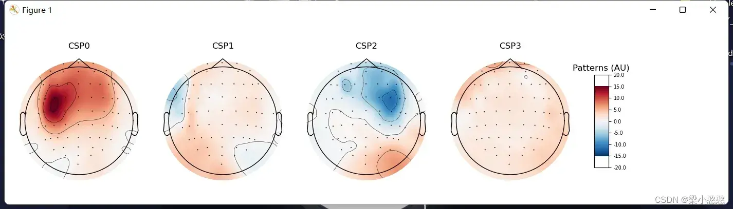
# plot CSP patterns estimated on full data for visualization
# csp提取特征,用于绘制CSP不同分量的模式图(地形图)
# 如果没有这一步csp.plot_patterns将不会执行
csp.fit_transform(epochs_data, labels)
# lay文件的存放路径,这个文件不是计算生成的,是mne库提供的点击分布描述文件在安装路径下(根据个人安装路径查找):
# D:\Program Files (x86)\Anaconda3\envs\pytorch_env\Lib\site-packages\mne\channels\data\layouts
layout = read_layout('EEG1005')
csp.plot_patterns(epochs.info, ch_type='eeg', units='Patterns (AU)', size=1.5)
# plt.show()
# #################################################################################################################
# # Verify the performance of the algorithm
sfreq = raw.info['sfreq'] # 获取数据的采样频率
w_length = int(sfreq * 0.5) # running classifier: window length
w_step = int(sfreq * 0.1) # running classifier: window step size
w_start = np.arange(0, epochs_data.shape[2] - w_length, w_step) # 每次滑动窗口的起始点
scores_windows = [] # 得分列表用于保存模型得分
for train_idx, test_idx in cv_split: # 交叉验证计算模型的性能
y_train, y_test = labels[train_idx], labels[test_idx] # 获取测试集和训练集数据
X_train = csp.fit_transform(epochs_data_train[train_idx], y_train) # 设置csp模型的参数,提取相关特征,用于后面的lda分类
# fit classifier
lda.fit(X_train, y_train) # 拟合lda模型
# running classifier: test classifier on sliding window
score_this_window = [] # 用于记录本次交叉验证的得分
for n in w_start:
X_test = csp.transform(epochs_data[test_idx][:, :, n:(n + w_length)]) # csp提取测试数据相关特征
score_this_window.append(lda.score(X_test, y_test)) # 获取测试数据得分
scores_windows.append(score_this_window) # 添加到总得分列表
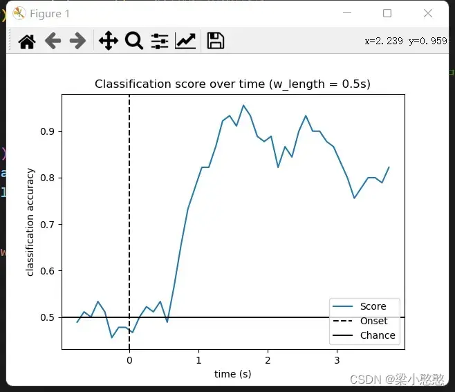
# Plot scores over time
w_times = (w_start + w_length / 2.) / sfreq + epochs.tmin # 设置绘图的时间轴,时间轴上的标志点为窗口的中间位置
# 绘制模型分类结果的性能图(得分的均值)
plt.figure()
plt.plot(w_times, np.mean(scores_windows, 0), label='Score')
plt.axvline(0, linestyle='--', color='k', label='Onset')
plt.axhline(0.5, linestyle='-', color='k', label='Chance')
plt.xlabel('time (s)')
plt.ylabel('classification accuracy')
plt.title('Classification score over time (w_length = {0}s)'.format(w_length/sfreq))
plt.legend(loc='lower right')
plt.show()
下面来看一下为什么测试数据集的时间窗口和训练数据集的时间窗口不一致也可以运行呢?lda的输入是经过csp提取后的特征,所以问题的重点是为什么csp的输入时间窗口可以不一致呢?
对于测试数据 来说,其特征向量
提取方式如下,并与
和
进行比较以确定第
次想象为想左或想右。
为提取的特征,是由
i计算得来,而
又是由矩阵
和
计算得来,看到这大概明白了,
是我们的投影矩阵,
是我们的输入数据,根据矩阵乘法的运算规则:前一个的列数等于后一个的行数,不难看出即使Xi的列数发生改变也不会影响计算。这里
的列数对应的就是时间窗口,我想这也就是为什么测试集的时间窗口和训练集的时间窗口可以不一致的原因吧。
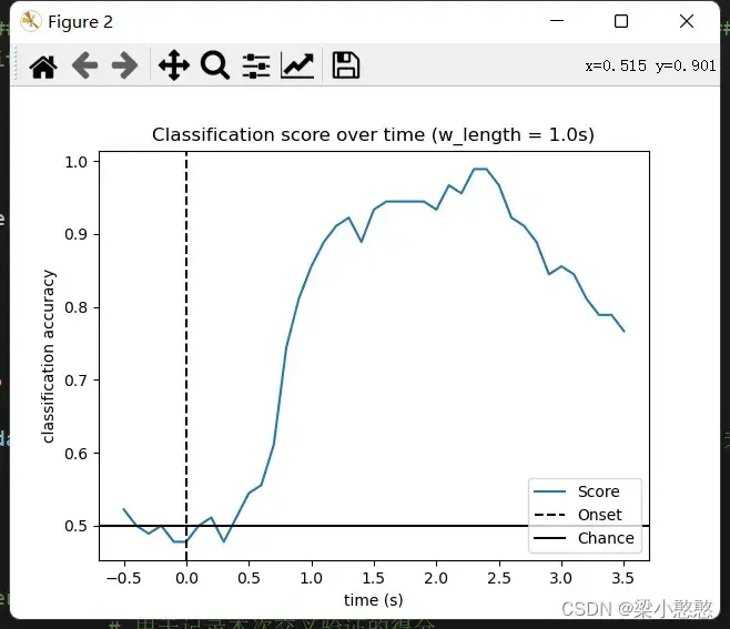
下面分别设置测试集时间窗口为秒(和训练集相同)和
秒,和上面
秒的时候相比,在这
种时间窗口中
秒的更加平稳,我想这也是其和训练集时间窗口一致的原因,毕竟测试集和训练集在数据维度上应该保持一致。不过这个特性倒是十分适合EEG这种具有时间序列特点的数据,这种使用方法或许在其他方面有意想不到的效果。
参考文章
特征提取丨共空间模式 Common Spatial Pattern (CSP)
文章出处登录后可见!