Python时间序列
时间序列(Time Series)是一种重要的结构化数据形式。时间序列的数据意义取决于具体的应用场景,主要有以下几种:
- 时间戳(timestamp):特定的时刻
- 固定时期(period):2007年1月或2010年全年
- 时间间隔(interval):由起始和结束时间戳表示。时期(period)可以被看作间隔的特例。
1. datetime模块
1.1 datetime对象
datetime.datetime对象(以下简称datetime对象)以毫秒形式存储日期和时间。datetime.timedelta表示datetime对象之间的时间差。
import pandas as pd
import numpy as np
from datetime import datetime,timedelta
%matplotlib inline
now = datetime.now() #now为datetime.datetime对象
now
输出:
datetime.datetime(2019, 10, 11, 15, 33, 5, 701305)
now.year,now.month,now.day
输出:
(2019, 10, 11)
delta = datetime.now()-datetime(2019,1,1) #delta为datetime.timedelta对象
datetime.now() + timedelta(12)
输出:
datetime.datetime(2023, 3, 10, 22, 13, 25, 3470)
1.2 字符串和datatime的相互转换
(1) 利用str或datetime.strftime方法(传入一个格式化字符串),datetime对象和pandas的Timestamp对象可以被格式化为字符串;datetime.strptime可以将字符串转换为日期。
stamp = datetime(2011,1,3)
stamp.strftime('%Y-%m-%d') #或str(stamp)
输出:
‘2011-01-03’
datetime.strptime('2019-10-01','%Y-%m-%d')
输出:
datetime.datetime(2019, 10, 1, 0, 0)
(2) 对于一些常见的日期格式,可以使用datautil中的parser.parse方法(不支持中文)
from dateutil.parser import parse
parse('2019-10-01') #形成datetime.datetime对象
输出:
datetime.datetime(2019, 10, 1, 0, 0)
(3) pandas的to_datetime方法可以解析多种不同的日期表示形式
import pandas as pd
datestrs = ['7/6/2019','8/6/2019']
dates = pd.to_datetime(datestrs) #将字符串列表转换为Timestamp对象
type(dates)
输出:
pandas.core.indexes.datetimes.DatetimeIndex
dates[0]
输出:
Timestamp(‘2019-07-06 00:00:00’)
2. 时间序列基础
pandas最基本的时间序列类型就是以时间戳(通常以Python字符串或datetime对象表示)为索引的Series。
时期(period)表示的是时间时区,比如数日、数月、数季、数年等。
from datetime import datetime

dates = [datetime(2019,1,1),datetime(2019,1,2),datetime(2019,1,5),datetime(2019,1,10),datetime(2019,2,10),datetime(2019,10,1)]

ts = pd.Series(np.random.randn(6),index = dates) #ts就成为一个时间序列,datetime对象实际上是被存放在一个DatetimeIndex中
ts
输出:
2019-01-01 1.175755
2019-01-02 -0.520842
2019-01-05 -0.678080
2019-01-10 0.195213
2019-02-10 2.201572
2019-10-01 0.115911
dtype: float64
dates = pd.DatetimeIndex(['2019/01/01','2019/01/02','2019/01/02','2019/5/01','3/15/2019']) #同一时间点上多个观测数据
dup_ts = pd.Series(np.arange(5),index = dates)
dup_ts
输出:
2019-01-01 0
2019-01-02 1
2019-01-02 2
2019-05-01 3
2019-03-15 4
dtype: int32
dup_ts.groupby(level = 0).count()
输出:
2019-01-01 1
2019-01-02 2
2019-03-15 1
2019-05-01 1
dtype: int64
pd.date_range可用于生成指定长度的DatetimeIndex
pd.date_range('2019/01/01','2019/2/1') #默认情况下产生按天计算的时间点。
输出:
DatetimeIndex([‘2019-01-01’, ‘2019-01-02’, ‘2019-01-03’, ‘2019-01-04’,
‘2019-01-05’, ‘2019-01-06’, ‘2019-01-07’, ‘2019-01-08’,
‘2019-01-09’, ‘2019-01-10’, ‘2019-01-11’, ‘2019-01-12’,
‘2019-01-13’, ‘2019-01-14’, ‘2019-01-15’, ‘2019-01-16’,
‘2019-01-17’, ‘2019-01-18’, ‘2019-01-19’, ‘2019-01-20’,
‘2019-01-21’, ‘2019-01-22’, ‘2019-01-23’, ‘2019-01-24’,
‘2019-01-25’, ‘2019-01-26’, ‘2019-01-27’, ‘2019-01-28’,
‘2019-01-29’, ‘2019-01-30’, ‘2019-01-31’, ‘2019-02-01’],
dtype=‘datetime64[ns]’, freq=‘D’)
pd.date_range('2010/01/01',periods = 30) # 传入起始或结束日期及一个表示时间段的数字。
输出:
DatetimeIndex([‘2010-01-01’, ‘2010-01-02’, ‘2010-01-03’, ‘2010-01-04’,
‘2010-01-05’, ‘2010-01-06’, ‘2010-01-07’, ‘2010-01-08’,
‘2010-01-09’, ‘2010-01-10’, ‘2010-01-11’, ‘2010-01-12’,
‘2010-01-13’, ‘2010-01-14’, ‘2010-01-15’, ‘2010-01-16’,
‘2010-01-17’, ‘2010-01-18’, ‘2010-01-19’, ‘2010-01-20’,
‘2010-01-21’, ‘2010-01-22’, ‘2010-01-23’, ‘2010-01-24’,
‘2010-01-25’, ‘2010-01-26’, ‘2010-01-27’, ‘2010-01-28’,
‘2010-01-29’, ‘2010-01-30’],
dtype=‘datetime64[ns]’, freq=‘D’)
pd.date_range('2010/01/01','2010/12/1',freq = 'BM') #传入BM(business end of month),生成每个月最后一个工作日组成的日期索引
输出:
DatetimeIndex([‘2010-01-29’, ‘2010-02-26’, ‘2010-03-31’, ‘2010-04-30’,
‘2010-05-31’, ‘2010-06-30’, ‘2010-07-30’, ‘2010-08-31’,
‘2010-09-30’, ‘2010-10-29’, ‘2010-11-30’],
dtype=‘datetime64[ns]’, freq=‘BM’)
pd.Series(np.arange(13),index = pd.date_range('2010/01/01','2010/1/3',freq = '4h'))
输出:
2010-01-01 00:00:00 0
2010-01-01 04:00:00 1
2010-01-01 08:00:00 2
2010-01-01 12:00:00 3
2010-01-01 16:00:00 4
2010-01-01 20:00:00 5
2010-01-02 00:00:00 6
2010-01-02 04:00:00 7
2010-01-02 08:00:00 8
2010-01-02 12:00:00 9
2010-01-02 16:00:00 10
2010-01-02 20:00:00 11
2010-01-03 00:00:00 12
Freq: 4H, dtype: int32
period_range可用于创建规则的时期范围
pd.Series(np.arange(10),index = pd.period_range('2019/1/1','2019/10/01',freq='M'))
输出:
2019-01 0
2019-02 1
2019-03 2
2019-04 3
2019-05 4
2019-06 5
2019-07 6
2019-08 7
2019-09 8
2019-10 9
Freq: M, dtype: int32
3. 重采样及频率转换
重采样(resampling)指的是将时间序列从一个频率转换到另一个频率的处理过程。
- 降采样(downsampling):将高频率数据聚合到低频率数据
- 升采样(upsampling):将低频率数据转换到高频率
rng = pd.date_range('2019/01/01',periods = 100,freq='D')
ts = pd.Series(np.random.randn(len(rng)),index=rng)
ts.resample('M').mean()
输出:
2019-01-31 0.011565
2019-02-28 -0.185584
2019-03-31 -0.323621
2019-04-30 0.043687
Freq: M, dtype: float64
ts.resample('M',kind='period').mean()
输出:
2019-01 0.011565
2019-02 -0.185584
2019-03 -0.323621
2019-04 0.043687
Freq: M, dtype: float64
rng = pd.date_range('2019/01/01',periods = 12,freq='T')
ts = pd.Series(np.random.randn(len(rng)),index=rng)
ts.resample('5min').sum()
输出:
2019-01-01 00:00:00 1.625143
2019-01-01 00:05:00 2.588045
2019-01-01 00:10:00 2.447725
Freq: 5T, dtype: float64
金融领域中有种时间序列聚合方式,称为OHLC重采样,即计算各面元的四个值:
- Open:开盘
- High:最高值
- Low:最小值
- Close:收盘
输出:
| open | high | low | close | |
|---|---|---|---|---|
| 2019-01-01 00:00:00 | -0.345952 | 1.120258 | -0.345952 | 1.120258 |
| 2019-01-01 00:05:00 | -0.106197 | 2.448439 | -1.014186 | -1.014186 |
| 2019-01-01 00:10:00 | 1.445036 | 1.445036 | 1.002688 | 1.002688 |
另一种降采样的办法是实用pandas的groupby方法。
rng = pd.date_range('2019/1/1',periods = 100,freq='D')
ts = pd.Series(np.arange(len(rng)), index = rng)
ts.resample('m').mean()
输出:
2019-01-31 15.0
2019-02-28 44.5
2019-03-31 74.0
2019-04-30 94.5
Freq: M, dtype: float64
ts.groupby(lambda x:x.month).mean()
输出:
1 15.0
2 44.5
3 74.0
4 94.5
dtype: float64
4. 时间序列可视化
需要加载stock.csv文件,该文件格式如下:
| AA | AAPL | GE | IBM | JNJ | MSFT | PEP | SPX | XOM | |
|---|---|---|---|---|---|---|---|---|---|
| 1990/2/1 0:00 | 4.98 | 7.86 | 2.87 | 16.79 | 4.27 | 0.51 | 6.04 | 328.79 | 6.12 |
| 1990/2/2 0:00 | 5.04 | 8 | 2.87 | 16.89 | 4.37 | 0.51 | 6.09 | 330.92 | 6.24 |
| 1990/2/5 0:00 | 5.07 | 8.18 | 2.87 | 17.32 | 4.34 | 0.51 | 6.05 | 331.85 | 6.25 |
| 1990/2/6 0:00 | 5.01 | 8.12 | 2.88 | 17.56 | 4.32 | 0.51 | 6.15 | 329.66 | 6.23 |
| 1990/2/7 0:00 | 5.04 | 7.77 | 2.91 | 17.93 | 4.38 | 0.51 | 6.17 | 333.75 | 6.33 |
close_px_all = pd.read_csv('datasets/stock.csv',parse_dates = True, index_col=0)
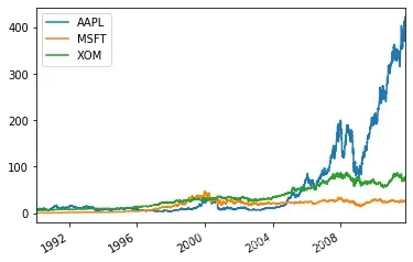
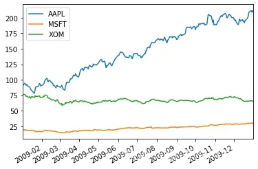
close_px = close_px_all[['AAPL','MSFT','XOM']]
close_px.plot() #'AAPL','MSFT','XOM'股价变化
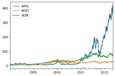
close_px.resample('B').ffill().plot() #填充工作日后,股价变化
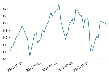
close_px.AAPL.loc['2011-01':'2011-03'].plot() #苹果公司2011年1月到3月每日股价
close_px.AAPL.loc['2011-01':'2011-03'].plot() #苹果公司2011年1月到3月每日股价
5. 窗口函数
5.1 移动窗口函数
移动窗口函数(moving window function)指在移动窗口(可带指数衰减权数)上计算的各种统计函数,也包括窗口不定长的函数(如指数加权移动平均)。 与其他统计函数一样,移动窗口函数会自动排除缺失值。
close_px.AAPL.plot()
close_px.AAPL.rolling(250).mean().plot()   #250日均线
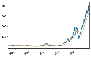
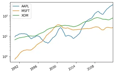
close_px.rolling(250).mean().plot(logy=True) #250日均线 对数坐标
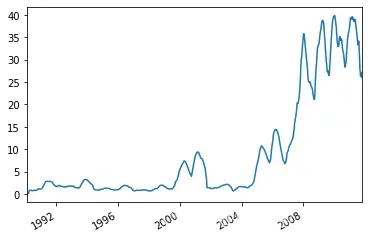
close_px.AAPL.rolling(250,min_periods=10).std().plot() #标准差
5.2 指数加权函数
指数加权函数:定义一个衰减因子(decay factor),以赋予近期的观测值拥有更大的权重。衰减因子常用时间间隔(span),可以使结果兼容于窗口大小等于时间间隔的简单移动窗口(simple moving window)函数。
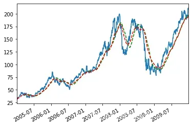
appl_px = close_px.AAPL['2005':'2009']
ma60 = appl_px.rolling(60,min_periods=50).mean()  #60日移动平均
ewma60 = appl_px.ewm(span = 60).mean()           #60日指数加权移动平均
appl_px.plot()
ma60.plot(c='g',style='k--')
ewma60.plot(c='r',style='k--')  #相对于普通移动平均,能“适应”更快的变化
5.3 二元移动窗口函数
相关系数和协方差等统计运算需要在两个时间序列上执行,如某只股票对某个参考指数(如标普500)的相关系数。
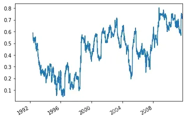
aapl_rets = close_px_all.AAPL['1992':].pct_change()
spx_rets = close_px_all.SPX.pct_change()
corr = aapl_rets.rolling(125,min_periods=100).corr(spx_rets) #APPL6个月回报与标准普尔500指数的相关系数
corr.plot()
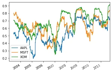
all_rets = close_px_all[['AAPL','MSFT','XOM']]['2003':].pct_change()
corr = all_rets.rolling(125,min_periods=100).corr(spx_rets) #3支股票月回报与标准普尔500指数的相关系数
corr.plot()
文章出处登录后可见!