一.PWC-Net 概述
PWC-Net 的网络模型在 CVPR,2018 由 NVIDIA 提出,发表文章为 《PWC-Net: CNNs for Optical Flow Using Pyramid, Warping, and Cost Volume》。与FlowNet2.0模型相比,PWCNet的大小缩小了17倍,训练成本更低且精确度稳定。此外,它在Sintel数据集(1024×436)图像上的运行速度大约为35 fps,是光流估计深度学习中非常基础且具有重要意义的一个网络模型。
FlowNet2.0 的提出证明了组织多个子网络结构构建更大型更复杂的光流估计网络可以提高光流估计的质量,但是这样做的后果就是使得训练复杂度和学习参数量成倍增加,并且容易出现过拟合问题。PWC-Net的核心优化点就在于如何在保证光流估计质量和精确性的前提下,尽可能地缩小训练体积。针对此问题,PWCNet将领域知识与深度学习相结合,利用多尺度特征来替换子网络串联,其设计遵循了三个简单而成熟的原则:金字塔特征提取(Pyramid),光流映射(Warping) 和匹配相关性成本代价衡量(Cost Volume),而其中Warping和Cost Volume都不包含任何学习参数,在保证网络行之有效的前提下极大减小了网络模型的体积。
二.PWC-Net 网络详解
1.网络结构
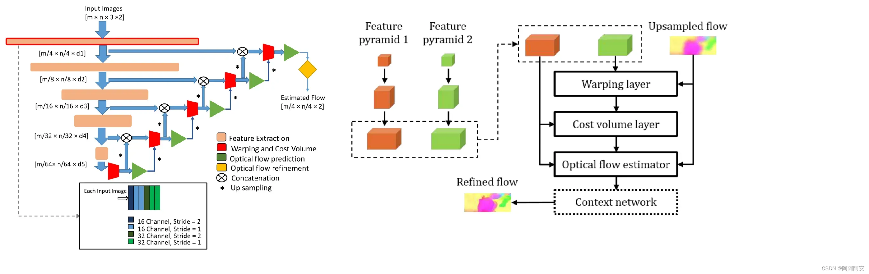
(1)Feature pyramid extractor
PWC-Net 使用金字塔结构分别对两张输入图像 进行多尺度的特征提取,生成特征表示的 L 层(L=6)金字塔,底部(第 0 层)是输入图像数据。随着金字塔层数的增加,使用卷积Filter对第l−1层金字塔层的特征进行下采样,特征尺寸逐步减小。从第一层到第六层,特征通道的数量分别为16、32、64、96、128和196。不同的特征尺度,可以认为具有不同感受野,能够提供更多的特征信息。
(2)Warping layer
Warping layer其实就是FlowNet中的Optical Flow Backwarping操作,用于将生成光流应用到目标图像上来生成映射后的图像数据。在第 l 层,我们使用来自第 l+1 层的 ×2 上采样光流(上采样的目的是将上层生成光流统一到当前尺寸)将第二张图像的特征backwarp到第一张图像特征视角,为后续匹配计算原始特征图像和warp特征图像做准备,该层不包含任何学习训练参数。
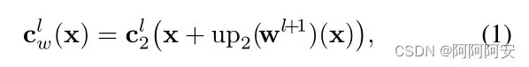
Warping 操作的目的,就是将上层较为粗糙的 flow 应用到下层的光流估计中,使每一层都是在上一层的基础上对光流进一步 refine,因此这种做法被称为 coarse-to-fine 方法,对于最顶层输入的 coarse flow 初始化为0或None。
(3)Cost volume layer
Cost volume 被定义为 image1 的特征与 warp 后 image2 的特征之间的相关性匹配成本量(代价),类似于 FlowNet 中的 Correlation Operation 。其定义公式如下:
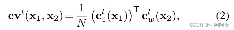
文章将 Correlation 的搜索范围限制为d,则该搜索窗的长宽为 D = 2d+1 ,Cost volume layer 输出成本量的维度为  , 其中
, 其中
# TensorFlow
class CostVolumeLayer(object):
    """ Cost volume module """
    def __init__(self, search_range = 4, name = 'cost_volume'):
        self.s_range = search_range
        self.name = name

    def __call__(self, features_0, features_0from1):
        with tf.name_scope(self.name) as ns:
            b, h, w, f = tf.unstack(tf.shape(features_0))
            cost_length = (2*self.s_range+1)**2

            get_c = partial(get_cost, features_0, features_0from1)
            cv = [0]*cost_length
            depth = 0
            for v in range(-self.s_range, self.s_range+1):
                for h in range(-self.s_range, self.s_range+1):
                    cv[depth] = get_c(shift = [v, h])
                    depth += 1

            cv = tf.stack(cv, axis = 3)
            cv = tf.nn.leaky_relu(cv, 0.1)
            return cv

# Pytorch
def corr(self, refimg_fea, targetimg_fea):
        maxdisp=4
        b,c,h,w = refimg_fea.shape
        targetimg_fea = F.unfold(targetimg_fea, (2*maxdisp+1,2*maxdisp+1), padding=maxdisp).view(b,c,2*maxdisp+1, 2*maxdisp+1**2,h,w)
        cost = refimg_fea.view(b,c,h,w)[:,:,np.newaxis, np.newaxis]*targetimg_fea.view(b,c,2*maxdisp+1, 2*maxdisp+1**2,h,w)
        cost = cost.sum(1)

        b, ph, pw, h, w = cost.size()
        cost = cost.view(b, ph * pw, h, w)/refimg_fea.size(1)
        return cost
(4)Optical flow estimator
该部分用于在每个特征层中输出预测的粗糙光流,一方面为多尺度训练损失提供flow,另一方面为下层提供refine的基础流。它是一个简单的多层 CNN 网络,其采用DenseNet架构,输入是本层计算的Cost volume、第一张图像在本层的提取特征(feature l)和上层的上采样光流(upflow) 的拼接,它的输出是第 l 层的预测光流 flow_l 。每个卷积层的特征通道数分别为128、128、96、64、32,2。
(5)Context network
传统的流方法通常使用上下文信息来对输出流进行后处理,目的是进一步细化流。因此,PWC-Net 使用一个称为上下文网络的子网络(Context network) 来有效地扩大每个输出单元的感受野大小。它从光流估计器中获取倒数第二层的估计流和特征,并输出一个细化的流。
它由 7 个卷积层组成,每个卷积层的卷积核为 3×3,不需要降低分辨率。这些层具有不同的膨胀系数(dilation),具有膨胀系数 k 的卷积层意味着层中filter的输入单元与层中filter的其他输入单元在垂直和水平方向上相距 k 个单位。具有大膨胀系数的卷积层扩大了每个输出单元的感受野,而不会产生大量的计算负担。每层的膨胀系数分别为 1、2、4、8、16、1 和 1。
2.更多细节
网络多尺度训练损失中的权重设置为 α6 = 0.32,α5 = 0.08,α4 = 0.02,α3 = 0.01,α2 = 0.005。权衡权重γ设置为0.0004。同时,网络的学习率设置为从 0.0001 开始,在 0.4M、0.6M、0.8M 和 1M 时将学习率减半迭代。
文章将 ground truth flow 缩放 20 倍并对其进行下采样以获得不同级别的监督信号(ground truth flow_l)。要注意的是,和FlowNet一样,文章并没有进一步缩放每个特征层上的监督信号。因此,需要在每个金字塔层中的warping layer缩放上采样流。比如第二层的warping layer中,我们在 image2 的warp之前需要将来自上层第三层(l=3)的上采样流数值扩大 5 倍(= 20/4)。文章使用 7 级金字塔并将  设置为 2,即模型输出四分之一分辨率的光流并使用双线性插值获得全分辨率光流(与FlowNet一致)。在Cost volume中,使用 4 个像素的搜索范围(range=4,d=9)来计算每个级别的成本量。
3.实现代码
from .correlation_package import correlation

# 特征金字塔提取器 Feature pyramid extractor
#   - 输入: image frame=(batchsize,channel=3,height,width)
#   - 输出: 六层提取特征 [tensorOne,...,tensorSix] (batchsize,channel,height,width)
class FeatureExtractor(nn.Module):
    def __init__(self):
        super(FeatureExtractor, self).__init__()

        self.moduleOne = nn.Sequential( #(batch,3,height,width) -> (batch,16,height/2,width/2)
            nn.Conv2d(in_channels=3, out_channels=16, kernel_size=3, stride=2, padding=1), #(batch,size,3) -> (batch,size/2,16)
            nn.LeakyReLU(inplace=False, negative_slope=0.1),
            nn.Conv2d(in_channels=16, out_channels=16, kernel_size=3, stride=1, padding=1),#(batch,size/2,16) -> (batch,size/2,16)
            nn.LeakyReLU(inplace=False, negative_slope=0.1),
            nn.Conv2d(in_channels=16, out_channels=16, kernel_size=3, stride=1, padding=1),#(batch,size/2,16) -> (batch,size/2,16)
            nn.LeakyReLU(inplace=False, negative_slope=0.1)
        )

        self.moduleTwo = nn.Sequential( #(batch,16,size/2) -> (batch,32,size/4)
            nn.Conv2d(in_channels=16, out_channels=32, kernel_size=3, stride=2, padding=1),
            nn.LeakyReLU(inplace=False, negative_slope=0.1),
            nn.Conv2d(in_channels=32, out_channels=32, kernel_size=3, stride=1, padding=1),
            nn.LeakyReLU(inplace=False, negative_slope=0.1),
            nn.Conv2d(in_channels=32, out_channels=32, kernel_size=3, stride=1, padding=1),
            nn.LeakyReLU(inplace=False, negative_slope=0.1)
        )

        self.moduleThr = nn.Sequential( #(batch,32,size/4) -> (batch,64,size/8)
            nn.Conv2d(in_channels=32, out_channels=64, kernel_size=3, stride=2, padding=1),
            nn.LeakyReLU(inplace=False, negative_slope=0.1),
            nn.Conv2d(in_channels=64, out_channels=64, kernel_size=3, stride=1, padding=1),
            nn.LeakyReLU(inplace=False, negative_slope=0.1),
            nn.Conv2d(in_channels=64, out_channels=64, kernel_size=3, stride=1, padding=1),
            nn.LeakyReLU(inplace=False, negative_slope=0.1)
        )

        self.moduleFou = nn.Sequential( #(batch,64,size/8) -> (batch,96,size/16)
            nn.Conv2d(in_channels=64, out_channels=96, kernel_size=3, stride=2, padding=1),
            nn.LeakyReLU(inplace=False, negative_slope=0.1),
            nn.Conv2d(in_channels=96, out_channels=96, kernel_size=3, stride=1, padding=1),
            nn.LeakyReLU(inplace=False, negative_slope=0.1),
            nn.Conv2d(in_channels=96, out_channels=96, kernel_size=3, stride=1, padding=1),
            nn.LeakyReLU(inplace=False, negative_slope=0.1)
        )

        self.moduleFiv = nn.Sequential( #(batch,,96,size/16) -> (batch,128,size/32)
            nn.Conv2d(in_channels=96, out_channels=128, kernel_size=3, stride=2, padding=1),
            nn.LeakyReLU(inplace=False, negative_slope=0.1),
            nn.Conv2d(in_channels=128, out_channels=128, kernel_size=3, stride=1, padding=1),
            nn.LeakyReLU(inplace=False, negative_slope=0.1),
            nn.Conv2d(in_channels=128, out_channels=128, kernel_size=3, stride=1, padding=1),
            nn.LeakyReLU(inplace=False, negative_slope=0.1)
        )

        self.moduleSix = nn.Sequential( #(batch,128,size/32) -> (batch,196,size/64)
            nn.Conv2d(in_channels=128, out_channels=196, kernel_size=3, stride=2, padding=1),
            nn.LeakyReLU(inplace=False, negative_slope=0.1),
            nn.Conv2d(in_channels=196, out_channels=196, kernel_size=3, stride=1, padding=1),
            nn.LeakyReLU(inplace=False, negative_slope=0.1),
            nn.Conv2d(in_channels=196, out_channels=196, kernel_size=3, stride=1, padding=1),
            nn.LeakyReLU(inplace=False, negative_slope=0.1)
        )

    def forward(self, tensorInput): #Input (batch,3,size)
        # get every layer
        tensorOne = self.moduleOne(tensorInput) #(batch,16,size/2)
        tensorTwo = self.moduleTwo(tensorOne) #(batch,32,size/4)
        tensorThr = self.moduleThr(tensorTwo) #(batch,64,size/8)
        tensorFou = self.moduleFou(tensorThr) #(batch,96,size/16)
        tensorFiv = self.moduleFiv(tensorFou) #(batch,128,size/32)
        tensorSix = self.moduleSix(tensorFiv) #(batch,196,size/64)
        # every layer get single by List
        return [ tensorOne, tensorTwo, tensorThr, tensorFou, tensorFiv, tensorSix ]

# warping layer 的另一种实现
class WarpingLayer(nn.Module):
    def __init__(self,batch_size: int, feature_height: int, feature_width: int) -> None:
        super(WarpingLayer, self).__init__()

        B, H, W = batch_size, feature_height, feature_width
        xx = torch.arange(0, W).view(1,-1).repeat(H,1)
        yy = torch.arange(0, H).view(-1,1).repeat(1,W)
        xx = xx.view(1,1,H,W).repeat(B,1,1,1)
        yy = yy.view(1,1,H,W).repeat(B,1,1,1)
        grid = torch.cat((xx,yy),1).float()

        self.register_buffer("grid", grid)

    def forward(self, x: torch.Tensor, flo: torch.Tensor):
        _, _, H, W = x.shape
        vgrid = self.grid + flo
        # scale grid to [-1,1]
        vgrid[:,0,:,:] = 2.0*vgrid[:, 0, :, :] / max(W-1, 1)-1.0
        vgrid[:,1,:,:] = 2.0*vgrid[:, 1, :, :] / max(H-1, 1)-1.0

        vgrid = vgrid.permute(0, 2, 3, 1)
        output = nn.functional.grid_sample(x, vgrid)
        return output

# 光流映射处理 Wraping layer(无学习参数)
class Backwarp(nn.Module):
    def __init__(self):
        super(Backwarp, self).__init__()

    # tensorInput : (batch,3,height,width)
    # tensorFlow : (batch,2,height,width)
    def forward(self, tensorInput, tensorFlow):
        # 1. mesh grid
        # tensorHorizontal (batch,1,height,width) -> 水平方向(x方向) 的像素坐标矩阵,并提前缩放到 [-1,1]范围
        tensorHorizontal = torch.linspace(-1.0, 1.0, tensorFlow.size(3)).view(1, 1, 1, tensorFlow.size(3)).expand(
            tensorFlow.size(0), -1, tensorFlow.size(2), -1)
        # tensorVertical (batch,1,height,width) -> 竖直方向(y方向) 的像素坐标矩阵,并提前缩放到 [-1,1]范围
        tensorVertical = torch.linspace(-1.0, 1.0, tensorFlow.size(2)).view(1, 1, tensorFlow.size(2), 1).expand(
            tensorFlow.size(0), -1, -1, tensorFlow.size(3))
        # 在 channel 方向合并为 tensorGrid (batch,2,height,width)
        tensorGrid = torch.cat([tensorHorizontal, tensorVertical], 1).cuda()
        # 2. create input
        tensorPartial = tensorFlow.new_ones(tensorFlow.size(0), 1, tensorFlow.size(2), tensorFlow.size(3)) #生成全1的 (batch,1,height,width) 的矩阵
        tensorInput = torch.cat([tensorInput, tensorPartial], 1)  # (batch,4,height,width)
        # Flow 也要相应进行缩放 [-1,1] -> flow*2/(size) -1.0
        tensorFlow = torch.cat([tensorFlow[:, 0:1, :, :] / ((tensorInput.size(3) - 1.0) / 2.0),
                                tensorFlow[:, 1:2, :, :] / ((tensorInput.size(2) - 1.0) / 2.0)], 1)
        # 3. get output
        tensorOutput = F.grid_sample(input=tensorInput, grid=(self.tensorGrid + tensorFlow).permute(0, 2, 3, 1),
                                    mode='bilinear', padding_mode='zeros')
        #- The auxiliary channel/mask that I introduced is used to zero out pixels
        #   that sample from the boundary where the original implementation yields zero but PyTorch's grid sampler yields something different.
        #   If you train a PWC-Net from scratch then you can safely remove this mechanism.
        #- Thanks @sniklaus, I'm training from scratch and I did notice a slight improvement in the losses when I removed that.
        #   Glad to know it is safe to remove for a fresh training.
        tensorMask = tensorOutput[:, -1:, :, :]
        tensorMask[tensorMask > 0.999] = 1.0
        tensorMask[tensorMask < 1.0] = 0.0

        return tensorOutput[:, :-1, :, :] * tensorMask

    # NVID backwarp 源码(好理解一些)
    # 简介:整个warp是从img2根据前向光流(前向光流是t -> t+1 帧的)warp到img1的过程,所以叫backwarp但我们最终算出来的还是前向flow(t - > t+1),光流进行可视化时,物体的轮廓和t时刻是一致的
    def backwarp(self, x, flo):
        """
        warp an image/tensor (im2) back to im1, according to the optical flow
        - 如果光流值完全准确,则warp后的图形应该与image1完全相同(warp image2 -> image1,所以是backwarp)

        x: [B, C, H, W] (im2)
        flo: [B, 2, H, W] flow

        """
        B, C, H, W = x.size()
        # create mesh grid :
        #   - meshgrid是 [x,y] 二维像素索引坐标的数组, 目的是建立两个grid之间的索引,为了方便光流的计算,这里我们生成一个与图像以及光流大小相同的 meshgrid
        #   - 先要明确 光流flow的值是相邻图像帧之间”像素坐标“的运动(亮度不变假设),因此我们要建立二维坐标xy的meshgrid方便光流warp过程计算
        xx = torch.arange(0, W).view(1, -1).repeat(H, 1)
        yy = torch.arange(0, H).view(-1, 1).repeat(1, W)
        xx = xx.view(1, 1, H, W).repeat(B, 1, 1, 1)
        yy = yy.view(1, 1, H, W).repeat(B, 1, 1, 1)
        grid = torch.cat((xx, yy), 1).float()

        if x.is_cuda:
            grid = grid.cuda()
        # - 将光流flow和meshgrid叠加,得到warp的初步结果。此时图二的每个像素坐标加上它的光流即为该像素点对应在图一的像素坐标
        # - 找到对应的像素点:若vgrid(x,y)的两个通道值为( m, n ),则表明output(x,y)的对应点RGB值应该在input的(m, n)处
        #       - 比如需要处理(2,3)这个坐标。那就查grid中坐标为(2,3)的值,假设为(3,3),那就把原图中(2,3)这个坐标上的值 赋给 输出(3,3)这个坐标(相对像素坐标运动)。
        # - 但是warp结果可能存在浮点数,因此我们需要进行插值的操作来得到“整数索引”所对应的值,这就是后面grid_sample的作用
        vgrid = Variable(grid) + flo

        # scale grid to [-1,1] ,为什么要这么变呢?是因为要配合grid_sample这个函数的使用
        # 将vgrid的取值范围归一化到[-1, 1]之间,用于grid_sample计算(在grid_sample函数内部实现中会重新映射回原始尺寸,不是多此一举可以统一输入尺寸单位)
        # 其中 比如[-1, -1]表示input左上角的像素的坐标,[1, 1]表示input右下角的像素的坐标
        vgrid[:, 0, :, :] = 2.0 * vgrid[:, 0, :, :].clone() / max(W - 1, 1) - 1.0
        vgrid[:, 1, :, :] = 2.0 * vgrid[:, 1, :, :].clone() / max(H - 1, 1) - 1.0

        # from B,2,H,W -> B,H,W,2,为什么要这么变呢?是因为要配合grid_sample这个函数的使用
        vgrid = vgrid.permute(0, 2, 3, 1)

        #  Given an input and a flow-field grid, computes the output using input values and pixel locations from grid.
        #       - input : 输入特征图
        #       - grid: grid包含输出特征图output的格网大小以及每个格网对应到输入特征图input的采样点位
        #  原理:
        #   - 简述: 对输入特征图的对应采样点位,上下左右四个角点值进行双线性插值计算,获取计算值作为output的采样结果(float非整数像素坐标直接向下取整floor然后采样计算)
        #   - 公式: output[x,y] = intput[left_top]*weight1 + input[left_bottom]*weight2 + input[right_top]*weight3 + input[right_bottom]*weight4 ( left_top... = Dir(floor(grid[x,y])) )
        #   - 关于光流flow方向: flow的方向是result图->source图, grid_sample(source, flow)得到result图. flow的方向其实是backward的
        output = nn.functional.grid_sample(x, vgrid)
        # mask用于过滤超出边界的点/异常点/四角点采样不全(采样信息不完整)的像素点
        # 作用详解:
        #   - 根据grid_simple函数的执行原理,即输出ouput(x,y) 的计算是通过grid对应的 grid(x,y)->(m,n)来获取inpput(m,n)四周的四个角点按比例系数求和进行采样
        #   - 若(m,n)四周四角点完整,则无论 (m,n) 是否为整数还是浮点数,采样公式在input全为1矩阵的时候采样求和结果都是1
        #       - 若四角点不完整,则<1,表示采样信息不完整应舍弃
        #       - 若目标月为越界点、异常点则<1,应舍弃
        #   - 因此,我们使用全1的mask来过滤异常点
        mask = torch.autograd.Variable(torch.ones(x.size())).cuda()
        mask = nn.functional.grid_sample(mask, vgrid)

        # if W==128:
        # np.save('mask.npy', mask.cpu().data.numpy())
        # np.save('warp.npy', output.cpu().data.numpy())
        mask[mask < 0.9999] = 0
        mask[mask > 0] = 1

        return output * mask

# Decoder Block
#   - wrap opteration
#   - costValume operation
#   - Optical flow estimator
class Decoder(nn.Module):
    #intLevel: 表示当前第几层的 Decoder Block
    def __init__(self, intLevel):
        super(Decoder, self).__init__()

        #1.记录每一层的 Optical flow estimator 初始输入的通道数
        #   - 顶层six : 81
        #   - 其他 : tensorVolume+tensorFirst+tensorFlow+tensorFeat
        intPrevious = [None, None, 81+32+2+2, 81+64+2+2, 81+96+2+2, 81+128+2+2, 81, None][intLevel+1]
        intCurrent = [None, None, 81+32+2+2, 81+64+2+2, 81+96+2+2, 81+128+2+2, 81, None][intLevel+0]
        if intLevel < 6:
            #   We scale the ground truth flow by 20 and down-sample it to obtain the supervision signals at different lev-els. Note that we do not further scale the supervision signalat each level, the same as [15].
            self.dblBackwarp = [None, None, None, 5.0, 2.5, 1.25, 0.625, None][intLevel + 1]

        #2.intLevel < 6: intLevel=6 表示顶层,顶层为默认设置(比如初始光流等),<6的层需要用到上层数据故需要设置
        #   (1)self.moduleUpflow:将上层光流上采样扩大到和本层input尺寸一致,(channel=2,Size) -> (channel=2,2*Size), 尺寸扩大两倍(和本层特征尺寸一致)
        if intLevel < 6:
            self.moduleUpflow = nn.ConvTranspose2d(in_channels=2, out_channels=2, kernel_size=4, stride=2, padding=1)
        #   (2)self.moduleUpfeat: 将上层给出的上下文信息压缩到2通道 in_channels=intPrevious + 128 + 128 + 96 + 64 + 32 -> 2,size -> 2*size 尺寸扩大两倍(和本层特征尺寸一致)
        if intLevel < 6:
            self.moduleUpfeat = nn.ConvTranspose2d(in_channels=intPrevious + 128 + 128 + 96 + 64 + 32, out_channels=2, kernel_size=4, stride=2, padding=1)
        #   (3)self.moduleBackward:wrap layer
        if intLevel < 6:
            self.moduleBackward = Backwarp()

        #3. self.moduleCorrelation: cost valume layer
        self.moduleCorrelation = correlation.Correlation()
        self.moduleCorreleaky = nn.LeakyReLU(inplace=False, negative_slope=0.1)

        #4. Optical flow estimator layer: [DenseNet] structer,the inputs to every convolu-tional layer are the output of and the input to its previouslayer.
        #   - (size) -> (size)
        self.moduleOne = nn.Sequential(
            nn.Conv2d(in_channels=intCurrent, out_channels=128, kernel_size=3, stride=1, padding=1),
            nn.LeakyReLU(inplace=False, negative_slope=0.1)
        )

        self.moduleTwo = nn.Sequential(
            nn.Conv2d(in_channels=intCurrent + 128, out_channels=128, kernel_size=3, stride=1, padding=1),
            nn.LeakyReLU(inplace=False, negative_slope=0.1)
        )

        self.moduleThr = nn.Sequential(
            nn.Conv2d(in_channels=intCurrent + 128 + 128, out_channels=96, kernel_size=3, stride=1, padding=1),
            nn.LeakyReLU(inplace=False, negative_slope=0.1)
        )

        self.moduleFou = nn.Sequential(
            nn.Conv2d(in_channels=intCurrent + 128 + 128 + 96, out_channels=64, kernel_size=3, stride=1, padding=1),
            nn.LeakyReLU(inplace=False, negative_slope=0.1)
        )

        self.moduleFiv = nn.Sequential(
            nn.Conv2d(in_channels=intCurrent + 128 + 128 + 96 + 64, out_channels=32, kernel_size=3, stride=1, padding=1),
            nn.LeakyReLU(inplace=False, negative_slope=0.1)
        )
        # (Size,channel) -> (Size,2)
        self.moduleSix = nn.Sequential(
            nn.Conv2d(in_channels=intCurrent + 128 + 128 + 96 + 64 + 32, out_channels=2, kernel_size=3, stride=1, padding=1)
        )

    def forward(self, tensorFirst, tensorSecond, objectPrevious):
        tensorFlow = None
        tensorFeat = None
        #1. wrap + costVolume 处理:使用上层输出光流 objectPrevious wrap tensorSecond 然后计算 costValume
        #   - 若objectPrevious is None:说明当前level是顶层(module six),默认初始光流为None则无需进行wrap,直接计算两个特征的costValume
        if objectPrevious is None:
            tensorFlow = None
            tensorFeat = None
            # tensorVolume = (batchsize,81,height,width): 196 channel => 81 channel (search range = 4,d = 9)
            tensorVolume = self.moduleCorreleaky(self.moduleCorrelation(tensorFirst, tensorSecond))
            # tensorFeat = (batchsize,81,height,width)
            tensorFeat = torch.cat([tensorVolume], 1)
        #   - 若objectPrevious is not None:说明是下流向层
        elif objectPrevious is not None:
            tensorFlow = self.moduleUpflow(objectPrevious['tensorFlow']) #上层光流上采样,扩大尺寸 -> 2通道
            tensorFeat = self.moduleUpfeat(objectPrevious['tensorFeat']) # 压缩上层上下文信息 -> 2通道
            # 计算costValume -> (batchsize,固定81通道,height,width)
            tensorVolume = self.moduleCorreleaky(self.moduleCorrelation(tensorFirst, self.moduleBackward(tensorSecond, tensorFlow*self.dblBackwarp)))
            # 将costValume、第一张图像帧、上层光流、上层 layer output(使用DenseNet架构) 拼接到一起作为后面Optical flow estimator输入 (input=81+本层特征channel+2+2)
            tensorFeat = torch.cat([tensorVolume, tensorFirst, tensorFlow, tensorFeat], 1)

        #2.光流预测 Optical flow estimator
        #   - DenseNet 架构:每一层 CNN 都将上一层layer的input和output拼接作为本层输入,构成前馈连接DenseNet
        #   - 网络入口初始输入是: 本层计算的tensorVolume+本层输入的tensorFirst+上层上采样tensorFlow+上层光流估计器中倒数第二层的输出的上下文信息 tensorFeat
        tensorFeat = torch.cat([self.moduleOne(tensorFeat), tensorFeat], 1) #(batchsize,128 + intcurrent,width,height)
        tensorFeat = torch.cat([self.moduleTwo(tensorFeat), tensorFeat], 1) #(batchsize,128 + 128+intcurrent,width,height)
        tensorFeat = torch.cat([self.moduleThr(tensorFeat), tensorFeat], 1) #(batchsize,96 + 128+128+intcurrent,width,height)
        tensorFeat = torch.cat([self.moduleFou(tensorFeat), tensorFeat], 1) #(batchsize,64 + 96+128+128+intcurrent,width,height)
        tensorFeat = torch.cat([self.moduleFiv(tensorFeat), tensorFeat], 1) #(batchsize,32 + 64+96+128+128+intcurrent,width,height) -- 光流估计器中获取倒数第二层的估计流和特征进入下层拼接为光流估计器初始输入(上下文)
        #   - 最后一层输出本层预测光流  (batchsize,2,width,height)
        tensorFlow = self.moduleSix(tensorFeat)

        return {
            'tensorFlow': tensorFlow,
            'tensorFeat': tensorFeat
        }

# Context 上下文后处理(细化光流) dilation -> 扩大感受野
#   - input: PWC-Net 输出倒数第二层的上下文信息 tensorFeat (batchsize,81+32+2+2 + 128+128+96+64+32,height/4,width/4)
#   - output: 光流细化矩阵 (batchsize,2,height/4,width/4)
class Refiner(nn.Module):
    def __init__(self):
        super(Refiner, self).__init__()

        self.moduleMain = nn.Sequential(
            nn.Conv2d(in_channels=81+32+2+2+128+128+96+64+32, out_channels=128, kernel_size=3, stride=1, padding=1,  dilation=1),#(batch,128,height/4,width/4)
            nn.LeakyReLU(inplace=False, negative_slope=0.1),
            nn.Conv2d(in_channels=128, out_channels=128, kernel_size=3, stride=1, padding=2,  dilation=2),#(batch,128,height/4,width/4)
            nn.LeakyReLU(inplace=False, negative_slope=0.1),
            nn.Conv2d(in_channels=128, out_channels=128, kernel_size=3, stride=1, padding=4,  dilation=4),#(batch,128,height/4,width/4)
            nn.LeakyReLU(inplace=False, negative_slope=0.1),
            nn.Conv2d(in_channels=128, out_channels=96, kernel_size=3, stride=1, padding=8,  dilation=8),#(batch,96,height/4,width/4)
            nn.LeakyReLU(inplace=False, negative_slope=0.1),
            nn.Conv2d(in_channels=96, out_channels=64, kernel_size=3, stride=1, padding=16,  dilation=16),#(batch,64,height/4,width/4)
            nn.LeakyReLU(inplace=False, negative_slope=0.1),
            nn.Conv2d(in_channels=64, out_channels=32, kernel_size=3, stride=1, padding=1,  dilation=1),#(batch,32,height/4,width/4)
            nn.LeakyReLU(inplace=False, negative_slope=0.1),
            nn.Conv2d(in_channels=32, out_channels=2, kernel_size=3, stride=1, padding=1,  dilation=1)#(batch,2,height/4,width/4)
        )

    def forward(self, tensorInput):
        return self.moduleMain(tensorInput)

# PWC-Net 总体架构网络
#   - 输入: 图像帧1+图像帧2 (batchsize,channel=3,height,width)
#   - 输出: 两帧图像之间的预测光流 (batch,channel=2,height/4,width/4)
class PWC_Net(nn.Module):
    def __init__(self, model_path=None):
        super(PWC_Net, self).__init__()
        self.model_path = model_path

        #1.初始化 特征金字塔提取器 moduleExtractor
        self.moduleExtractor = FeatureExtractor()
        #2.初始化 Decoder Block (五层)
        self.moduleTwo = Decoder(2)
        self.moduleThr = Decoder(3)
        self.moduleFou = Decoder(4)
        self.moduleFiv = Decoder(5)
        self.moduleSix = Decoder(6)
        #3.初始化 上下文细化网络(在倒数第二层起作用)
        self.moduleRefiner = Refiner()
        #4.加载训练好的模型参数
        if self.model_path != None:
            self.load_state_dict(torch.load(self.model_path))

    def forward(self, tensorFirst, tensorSecond):
        #1. 两张图像帧构造两个特征金字塔 tensorImage=(batchsize,channel,height,width)
        #   - tensorFirst : [tensorOne...]
        #   - tensorSecond : [tensorOne...]
        tensorFirst = self.moduleExtractor(tensorFirst)
        tensorSecond = self.moduleExtractor(tensorSecond)
        #2. 光流预测在特征层反向流动
        #- 输入:
        #   - 第一帧图像的当前层特征
        #   - 第二帧图像的当前层特征
        #   - 上层输出光流 + 上下文特征信息(初始/顶层为None)
        #- 输出:
        #   - 当前层的预测光流+上下文信息(光流估计器中获取倒数第二层的估计流和特征)
        objectEstimate = self.moduleSix(tensorFirst[-1], tensorSecond[-1], None)
        flow6 = objectEstimate['tensorFlow']
        objectEstimate = self.moduleFiv(tensorFirst[-2], tensorSecond[-2], objectEstimate)
        flow5 = objectEstimate['tensorFlow']
        objectEstimate = self.moduleFou(tensorFirst[-3], tensorSecond[-3], objectEstimate)
        flow4 = objectEstimate['tensorFlow']
        objectEstimate = self.moduleThr(tensorFirst[-4], tensorSecond[-4], objectEstimate)
        flow3 = objectEstimate['tensorFlow']
        objectEstimate = self.moduleTwo(tensorFirst[-5], tensorSecond[-5], objectEstimate) #(batchsize,2 + 32+64+96+128+128+intcurrent,height/4,width/4)
        flow2 = objectEstimate['tensorFlow']
        #3. 细化+输出 flow=(batchsize,2,height/4,width/4)
        #   当然,作者发现继续使用upconvolutional,对特征图的细节恢复作用已不明显,为了避免更多计算开销,后续使用双线性插值(bilinear upsampling)更好。
        flow2 = flow2 + self.moduleRefiner(objectEstimate['tensorFeat'])
        # 多尺度训练损失
        if self.training:
            return flow2, flow3, flow4, flow5, flow6
        else:
            return flow2
三.网络训练
PWC-Net 的训练过程与 FlowNet 类似,只是注意学习率 lr 的迭代策略即可,部分示例代码如下(此处仅作参考,不保证准确性):
# learning rate schedule
def adjust_learning_rate(optimizer, total_iters):
    if lr_schedule == 'slong':
        if total_iters < 200000:
            lr = baselr
        elif total_iters < 300000:
            lr = baselr / 2.
        elif total_iters < 400000:
            lr = baselr / 4.
        elif total_iters < 500000:
            lr = baselr / 8.
        elif total_iters < 600000:
            lr = baselr / 16.
    if lr_schedule == 'rob_ours':
        if total_iters < 30000:
            lr = baselr
        elif total_iters < 40000:
            lr = baselr / 2.
        elif total_iters < 50000:
            lr = baselr / 4.
        elif total_iters < 60000:
            lr = baselr / 8.
        elif total_iters < 70000:
            lr = baselr / 16.
        elif total_iters < 100000:
            lr = baselr
        elif total_iters < 110000:
            lr = baselr / 2.
        elif total_iters < 120000:
            lr = baselr / 4.
        elif total_iters < 130000:
            lr = baselr / 8.
        elif total_iters < 140000:
            lr = baselr / 16.
    for param_group in optimizer.param_groups:
        param_group['lr'] = lr

# EPE Loss
def EPE(input_flow, target_flow):
    return torch.norm(target_flow - input_flow, p=2, dim=1).mean()


def realEPE(output, target):
    b, _, h, w = target.size()
    upsampled_output = F.interpolate(output, (h, w), mode='bilinear', align_corners=False)
    return EPE(upsampled_output, target)


# 多尺度训练损失(flow2~flow6的EPE损失求和权重不同)
def multiscaleEPE(network_output, target_flow, weights=None):
    def one_scale(output, target):
        b, _, h, w = output.size()
        # 为防止 target 和 output 尺寸不一,使用插值方式来统一图像尺寸
        target_scaled = F.interpolate(target, (h, w), mode='area')
        return EPE(output, target_scaled)

    loss = 0
    for output, weight in zip(network_output, weights):
        loss += weight * one_scale(output, target_flow)
    return loss

# 单轮训练
def train(train_loader, model, optimizer, epoch):
    global n_iter, args
    # training weight for each scale, from highest resolution (flow2) to lowest (flow6)
    multiscale_weights = [0.005, 0.01, 0.02, 0.08, 0.32]
    # value by which flow will be divided. Original value is 20 but 1 with batchNorm gives good results
    div_flow = 20
    losses = 0.0
    flow2_EPEs = 0.0

    epoch_size = len(train_loader) if args.epoch_size == 0 else min(len(train_loader), args.epoch_size)

    # switch to train mode
    model.train()

    for i, (input, target) in enumerate(train_loader):
        target = target.to(device)
        input = torch.cat(input,1).to(device)

        # compute output
        output = model(input)
        # compute loss
        loss = multiscaleEPE(output, target, weights=multiscale_weights)  # 多尺度训练损失
        flow2_EPE = realEPE(div_flow * output[0], target)  # 最终输出光流flow2的单独损失
        # record loss and EPE
        losses += loss.item()
        flow2_EPEs += flow2_EPE.item()

        # compute gradient and do optimization step
        optimizer.zero_grad()
        loss.backward()
        optimizer.step()

        n_iter += 1
        if i >= epoch_size:
            break

    return losses, flow2_EPEs

if __name__ == '__main__':
    global total_iters
    # params set
    batch_size = 4 * ngpus
    lr_schedule = 'rob_ours'
    baselr = 1e-3
    worker_mul = int(2)
    # get dataLoader
    TrainImgLoader = torch.utils.data.DataLoader(
        data_inuse,
        batch_size=batch_size, shuffle=True, num_workers=worker_mul * batch_size, drop_last=True,
        worker_init_fn=_init_fn, pin_memory=True)
    # get model
    model = pwcnet()
    model.cuda()
    # get optimizer
    optimizer = optim.Adam(model.parameters(), lr=1e-4, betas=(0.9, 0.999), amsgrad=False)
    # epochs train
    for epoch in range(1, args.epochs + 1):
        total_train_loss = 0
        total_train_aepe = 0

        # training loop
        for batch_idx, (imgL, imgR, flow_gt) in enumerate(TrainImgLoader):
            # adjust learning rate
            if batch_idx % 100 == 0:
                adjust_learning_rate(optimizer, total_iters)
            # one train and loss
            train_loss, train_EPE = train(TrainImgLoader,model,optimizer,epoch)
            print('Iter %d training loss = %.3f , time = %.2f' % (batch_idx, train_loss, time.time() - start_time))
            total_train_loss += train_loss
            total_train_aepe += train_EPE

            total_iters += 1
文章出处登录后可见!