很早之前看过这篇论文,但是当时还是以多线激光雷达为主,最近又回到了2D激光里程计,所以有重新看了这部分代码,顺便记录一下!
之前的原理部分可参考:RF2O激光里程计算法原理
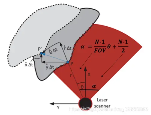
设为范围扫描,其中
是时间,
是扫描坐标,N是扫描的大小。 任何点P相对于连接到传感器的局部参考系的位置由其极坐标
给出,如果从激光雷达扫描点P,则
如下所示,其中FOV为扫描仪的视野:
1.CMakeLists 起飞
先从CMakeLists开始吧~
find_package(catkin REQUIRED COMPONENTS
  roscpp
  rospy
  nav_msgs
  sensor_msgs
  std_msgs
  tf
)
find_package(Boost REQUIRED COMPONENTS system)
find_package(cmake_modules REQUIRED)
find_package(Eigen REQUIRED)
find_package(MRPT REQUIRED base obs maps slam)
因为以后打算去ROS,所以比较关注项目的依赖。这里还有一个tf,貌似比较简单,还有一个不熟悉的库MRPT,官网介绍如下:
移动机器人编程工具包 (MRPT) 是一个广泛的、跨平台的开源 C++ 库,旨在帮助机器人研究人员设计和实施(主要)在同步定位和建图 (SLAM)、计算机视觉和运动规划(避障)。优点是代码的效率和可重用性。
这些库用于轻松管理 3D(6D) 几何的类、许多预定义变量(点和位姿、路标、地图)的概率密度函数 (pdf)、贝叶斯估计(卡尔曼滤波器、粒子滤波器)、图像处理、路径规划和障碍物躲避,所有类型的地图(点,栅格地图,路标,…)等的 3D 可视化。
高效地收集、操作和检查非常大的机器人数据集 (Rawlogs) 是 MRPT 的另一个目标,由多个类和应用程序支持。
这里怎么用只有看代码才能知道,所有代码都包含在一个cpp中,对!
add_executable(rf2o_laser_odometry_node src/CLaserOdometry2D.cpp)
int main(int argc, char** argv)
{
    ros::init(argc, argv, "RF2O_LaserOdom");
    CLaserOdometry2D myLaserOdom;
    ROS_INFO("initialization complete...Looping");
    ros::Rate loop_rate(myLaserOdom.freq);
    while (ros::ok()) {
        ros::spinOnce();        //Check for new laser scans
        if( myLaserOdom.is_initialized() && myLaserOdom.scan_available() ) {
            //Process odometry estimation
            myLaserOdom.odometryCalculation();
        }
        else {
            ROS_WARN("Waiting for laser_scans....") ;
        }
        loop_rate.sleep();
    }
    return(0);
}
2.main 函数
首先是创建一个新的激光里程计对象。在该类的构造函数中,定义了激光数据的topic名称:/laser_scan、发布的tf坐标系关系/base_link、/odom、发布的频率freq是一些基本参数。然后是接收和发送的定义。
在main函数的主循环中,需要在计算激光里程表之前判断是否初始化Init()以及是否有新的激光数据。相当于两个线程运行,一个通过消息回调接收数据,当有新数据时,主循环会调用激光里程计计算位置信息。
3.回调函数与数据初始化
void CLaserOdometry2D::LaserCallBack(const sensor_msgs::LaserScan::ConstPtr& new_scan) {
    //Keep in memory the last received laser_scan
    last_scan = *new_scan;
    //Initialize module on first scan
    if (first_laser_scan) {
        Init();
        first_laser_scan = false;
    }
    else {
        //copy laser scan to internal variable
        for (unsigned int i = 0; i<width; i++)
            range_wf(i) = new_scan->ranges[i];
        new_scan_available = true;
    }
}
在回调函数LaserCallBack中,什么都不做,初始化一帧Init(),然后在range_wf中存储以下数据,用于计算位置信息。
void CLaserOdometry2D::Init()
{
    // Got an initial scan laser, obtain its parametes 在第一帧激光数据,定义其参数
    ROS_INFO("Got first Laser Scan .... Configuring node");
    width = last_scan.ranges.size();    // Num of samples (size) of the scan laser 激光雷达的激光束数
    cols = width;						// Max reolution. Should be similar to the width parameter
    fovh = fabs(last_scan.angle_max - last_scan.angle_min); // Horizontal Laser's FOV 激光雷达的水平视角
    ctf_levels = 5;                     // Coarse-to-Fine levels 设置一个由粗到细的 变换矩阵
    iter_irls = 5;                      //Num iterations to solve iterative reweighted least squares 最小二乘的迭代次数

    // Set laser pose on the robot (through tF) 通过 TF 设置激光雷达在小车上的位置
    // This allow estimation of the odometry with respect to the robot base reference system.
    // 得到的里程计信息是相对于机器人坐标系
    mrpt::poses::CPose3D LaserPoseOnTheRobot;
    tf::StampedTransform transform;
    try {
    	 // 得到激光坐标系 到 机器人坐标系的 转换关系
        tf_listener.lookupTransform("/base_link", last_scan.header.frame_id, ros::Time(0), transform);
    }
    catch (tf::TransformException &ex) {
        ROS_ERROR("%s",ex.what());
        ros::Duration(1.0).sleep();
    }

    //TF:transform -> mrpt::CPose3D (see mrpt-ros-bridge)
    const tf::Vector3 &t = transform.getOrigin(); // 平移
    LaserPoseOnTheRobot.x() = t[0];
    LaserPoseOnTheRobot.y() = t[1];
    LaserPoseOnTheRobot.z() = t[2];
    const tf::Matrix3x3 &basis = transform.getBasis(); // 旋转
    mrpt::math::CMatrixDouble33 R;
    for(int r = 0; r < 3; r++)
        for(int c = 0; c < 3; c++)
            R(r,c) = basis[r][c];
    LaserPoseOnTheRobot.setRotationMatrix(R);

    //Set the initial pose 设置激光雷达的初始位姿,在机器人坐标系下
    laser_pose = LaserPoseOnTheRobot;
    laser_oldpose = LaserPoseOnTheRobot;

    // Init module 初始化模型
    //-------------
    range_wf.setSize(1, width);

    //Resize vectors according to levels 初始化 由粗到精 的变化矩阵
    transformations.resize(ctf_levels);
    for (unsigned int i = 0; i < ctf_levels; i++)
        transformations[i].resize(3, 3);

    //Resize pyramid 调整金字塔大小
    unsigned int s, cols_i;
    const unsigned int pyr_levels = round(log2(round(float(width) / float(cols)))) + ctf_levels; // 金字塔层数,
    range.resize(pyr_levels);
    range_old.resize(pyr_levels);
    range_inter.resize(pyr_levels);
    xx.resize(pyr_levels);
    xx_inter.resize(pyr_levels);
    xx_old.resize(pyr_levels);
    yy.resize(pyr_levels);
    yy_inter.resize(pyr_levels);
    yy_old.resize(pyr_levels);
    range_warped.resize(pyr_levels);
    xx_warped.resize(pyr_levels);
    yy_warped.resize(pyr_levels);

    for (unsigned int i = 0; i < pyr_levels; i++) {
        s = pow(2.f, int(i));
        //每一层的尺度,1 - 0.5 - 0.25 - 0.125 - 0.0625
        cols_i = ceil(float(width) / float(s));

        range[i].resize(1, cols_i);
        range_inter[i].resize(1, cols_i);
        range_old[i].resize(1, cols_i);
        range[i].assign(0.0f);
        range_old[i].assign(0.0f);
        xx[i].resize(1, cols_i);
        xx_inter[i].resize(1, cols_i);
        xx_old[i].resize(1, cols_i);
        xx[i].assign(0.0f);
        xx_old[i].assign(0.0f);
        yy[i].resize(1, cols_i);
        yy_inter[i].resize(1, cols_i);
        yy_old[i].resize(1, cols_i);
        yy[i].assign(0.f);
        yy_old[i].assign(0.f);

        if (cols_i <= cols) {
            range_warped[i].resize(1, cols_i);
            xx_warped[i].resize(1, cols_i);
            yy_warped[i].resize(1, cols_i);
        }
    }

    dt.resize(1, cols);
    dtita.resize(1, cols);
    normx.resize(1, cols);
    normy.resize(1, cols);
    norm_ang.resize(1, cols);
    weights.setSize(1, cols);
    null.setSize(1, cols);
    null.assign(0);
    cov_odo.assign(0.f);

    fps = 1.f;		//In Hz
    num_valid_range = 0; // 有效的激光距离数据个数

    // Compute gaussian mask 计算高斯掩码  [1/16,1/4,6/16,1/4,1/16] 用于计算加权平均值
    g_mask[0] = 1.f / 16.f; g_mask[1] = 0.25f; g_mask[2] = 6.f / 16.f; g_mask[3] = g_mask[1]; g_mask[4] = g_mask[0];

    kai_abs.assign(0.f);
    kai_loc_old.assign(0.f);

    module_initialized = true; // 模型初始化完成
    last_odom_time = ros::Time::now();
}
一般来说,在初始化过程中,会加载激光数据的参数信息,并初始化一些容器。现在计算所需的参数、容器和激光数据就像待宰的羔羊,所以下一步要开始了。
4.计算激光里程计的主循环
下面是main函数中的odometryCalculation,开始计算激光里程表。在原始代码中,注释也很清楚。
4.1 创建图像金字塔 createImagePyramid
首先是创建图像金字塔createImagePyramid,
void CLaserOdometry2D::createImagePyramid() {
	const float max_range_dif = 0.3f; // 最大的距离差值
	//Push the frames back 更新数据
	range_old.swap(range);
	xx_old.swap(xx);
	yy_old.swap(yy);

  // 金字塔的层数与里程计计算中使用的层数不匹配(因为我们有时希望以较低的分辨率完成)
  unsigned int pyr_levels = round(log2(round(float(width)/float(cols)))) + ctf_levels;

  //Generate levels 开始创建金字塔
  for (unsigned int i = 0; i<pyr_levels; i++) {
    unsigned int s = pow(2.f,int(i)); // 每次缩放 2 倍
    cols_i = ceil(float(width)/float(s));
    const unsigned int i_1 = i-1; // 上一层

    //First level -> Filter (not downsampling);
    if (i == 0) { // i = 0 第一层进行滤波
      for (unsigned int u = 0; u < cols_i; u++) {
        const float dcenter = range_wf(u);
        //Inner pixels  内部像素的处理, u从第三列开始到倒数第三列
        if ((u>1)&&(u<cols_i-2)) {
          if (dcenter > 0.f) {	// 当前激光距离大于0,一般都满足
            float sum = 0.f; // 累加量,用于计算加权平均值
            float weight = 0.f; // 权重
            for (int l=-2; l<3; l++) { // 取附近五个点
              const float abs_dif = abs(range_wf(u+l)-dcenter); // 该点附近的五个点的距离,与当前点距离的绝对误差
              if (abs_dif < max_range_dif) { // 误差满足阈值
                const float aux_w = g_mask[2+l]*(max_range_dif - abs_dif); // 认为越靠近该点的 权重应该最大,加权平均值
                weight += aux_w;
                sum += aux_w*range_wf(u+l);
              }
            }
          range[i](u) = sum/weight;
          }
          else // 否则当前激光距离设为0
            range[i](u) = 0.f;
        }

        //Boundary 下面对边界像素的处理
        else {
          if (dcenter > 0.f){	 // 判断激光距离是否合法
            float sum = 0.f;
            float weight = 0.f;
            for (int l=-2; l<3; l++)	{ // 计算加权平均值,只不过需要判断是否会越界
              const int indu = u+l;
              if ((indu>=0)&&(indu<cols_i)){
                const float abs_dif = abs(range_wf(indu)-dcenter);
                if (abs_dif < max_range_dif){
                  const float aux_w = g_mask[2+l]*(max_range_dif - abs_dif);
                  weight += aux_w;
                  sum += aux_w*range_wf(indu);
                }
              }
            }
            range[i](u) = sum/weight;
          }
          else
            range[i](u) = 0.f;
        }
      }
    }
    //-----------------------------------------------------------------------------
    // 从第二层开始,做下采样,同样也是分为内部点,和边界点进行处理,原理与第一层相同,计算加权平均值
    // 不过值得注意的是,从第二层开始 使用的数据是上一层下采样后的数据,即range[i_1],因此每次计算都会缩小2倍。
    // ......
  }
}
以上呢,就计算得到了每一层金字塔内所包含的点云位置,借用百度百科中的一张图,可以直观的看出图像金字塔的效果。不过这里是一个2D的金字塔,相当与降低了分辨率,用附近的点云距离,通过加权平均值算出一个”代表”。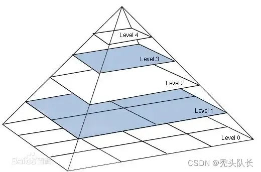
4.2 金字塔处理的八个步骤
然后,金字塔每一层的处理分为八个步骤,这也是核心部分。首先介绍一下整个流程,后面会详细介绍各个功能。
void CLaserOdometry2D::odometryCalculation()
{
    m_clock.Tic();
    createImagePyramid();  // 计算金字塔

    //Coarse-to-fine scheme // 从金字塔的顶端开始开始
    for (unsigned int i=0; i<ctf_levels; i++) {
        //Previous computations  首先把旋转矩阵初始化
        transformations[i].setIdentity();

        level = i; // 记录目前计算进度,因为上一层的计算会当作下一层的初值,由粗到细的迭代
        unsigned int s = pow(2.f,int(ctf_levels-(i+1)));  // 从金字塔的最顶端开始,所以需要做一下处理,计算出最高层的缩放系数
        cols_i = ceil(float(cols)/float(s));  // 缩放后的数据长度
        image_level = ctf_levels - i + round(log2(round(float(width)/float(cols)))) - 1; // 当前需要处理的金字塔层数

        //1. Perform warping
        if (i == 0) {
            range_warped[image_level] = range[image_level];
            xx_warped[image_level] = xx[image_level];
            yy_warped[image_level] = yy[image_level];
        }
        else
            performWarping();

        //2. Calculate inter coords
        calculateCoord();

        //3. Find null points
        findNullPoints();

        //4. Compute derivatives
        calculaterangeDerivativesSurface();

        //5. Compute normals
        //computeNormals();

        //6. Compute weights
        computeWeights();

        //7. Solve odometry
        if (num_valid_range > 3) {
            solveSystemNonLinear();
            //solveSystemOneLevel();    //without robust-function
        }

        //8. Filter solution
        filterLevelSolution();
    }

    m_runtime = 1000*m_clock.Tac();
    ROS_INFO("Time odometry (ms): %f", m_runtime);

    //Update poses
    PoseUpdate();
    new_scan_available = false;     //avoids the possibility to run twice on the same laser scan
}
4.2.1 calculateCoord
我们按照处理顺序。最高层不进行数据转换部分,所以直接计算坐标。
void CLaserOdometry2D::calculateCoord()
{
	for (unsigned int u = 0; u < cols_i; u++) // 遍历该层的所有数据信息
	{
	  // 如果上一帧该层的数据 或者这一帧数据 为0就不处理
		if ((range_old[image_level](u) == 0.f) || (range_warped[image_level](u) == 0.f))
		{
			range_inter[image_level](u) = 0.f;
			xx_inter[image_level](u) = 0.f;
			yy_inter[image_level](u) = 0.f;
		}
		else // 否则 取两者均值
		{
			range_inter[image_level](u) = 0.5f*(range_old[image_level](u) + range_warped[image_level](u));
			xx_inter[image_level](u) = 0.5f*(xx_old[image_level](u) + xx_warped[image_level](u));
			yy_inter[image_level](u) = 0.5f*(yy_old[image_level](u) + yy_warped[image_level](u));
		}
	}
}
4.2.2 findNullPoints
找到一些距离为0的点,因为在之前金字塔缩放的时候,距离小与0的不合法激光数据都被置为0了。
void CLaserOdometry2D::findNullPoints()
{
	//Size of null matrix is set to its maximum size (constructor)
	// 记录空值的矩阵是 最大的数据大小,也就是和最底层的金字塔一样,不会访问越界
	num_valid_range = 0;
	for (unsigned int u = 1; u < cols_i-1; u++)
	{
		if (range_inter[image_level](u) == 0.f)
			null(u) = 1;
		else
		{
			num_valid_range++; // 记录有效激光点的个数
			null(u) = 0;
		}
	}
}
4.2.3 Compute derivatives
我们的算法特别关注range梯度的计算。通常,使用固定的离散公式来近似扫描或图像梯度。在range数据的情况下,这种策略会导致对象边界处的梯度值非常高,这并不代表这些对象上的真实梯度。作为替代方案,我们使用关于环境几何形状的自适应公式。该公式使用连续观测(点)之间的 2D 距离对扫描中的前向和后向导数进行加权:
// 计算相邻两点的 距离差值
for (unsigned int u = 0; u < cols_i-1; u++)
{
	const float dist = square(xx_inter[image_level](u+1) - xx_inter[image_level](u))
						+ square(yy_inter[image_level](u+1) - yy_inter[image_level](u));
	if (dist  > 0.f)
		rtita(u) = sqrt(dist);
}
//Spatial derivatives
for (unsigned int u = 1; u < cols_i-1; u++)
dtita(u) = (rtita(u-1)*(range_inter[image_level](u+1)-range_inter[image_level](u)) + rtita(u)*
    (range_inter[image_level](u) - range_inter[image_level](u-1)))/(rtita(u)+rtita(u-1));
// 第一对点 和 最后一对点 单独赋值
dtita(0) = dtita(1);
dtita(cols_i-1) = dtita(cols_i-2);
因此,最近的邻居总是对梯度计算贡献更多,而远点几乎不影响它。在两个邻居近似等距的情况下,所提出的公式等价于中心差分法。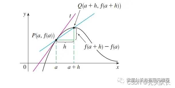
	//Temporal derivative 对时间求导得到速度
	for (unsigned int u = 0; u < cols_i; u++)
		dt(u) = fps*(range_warped[image_level](u) - range_old[image_level](u));
4.2.4 computeNormals
void CLaserOdometry2D::computeNormals()
{
	normx.assign(0.f);
	normy.assign(0.f);
	norm_ang.assign(0.f);

	const float incr_tita = fovh/float(cols_i-1);
	for (unsigned int u=0; u<cols_i; u++)
	{
		if (null(u) == 0.f)
		{
			const float tita = -0.5f*fovh + float(u)*incr_tita;
			const float alfa = -atan2(2.f*dtita(u), 2.f*range[image_level](u)*incr_tita);
			norm_ang(u) = tita + alfa;
			if (norm_ang(u) < -M_PI)
				norm_ang(u) += 2.f*M_PI;
			else if (norm_ang(u) < 0.f)
				norm_ang(u) += M_PI;
			else if (norm_ang(u) > M_PI)
				norm_ang(u) -= M_PI;

			normx(u) = cos(tita + alfa);
			normy(u) = sin(tita + alfa);
		}
	}
}
4.2.5 computeWeights
根据代码,我们推导出公式,其中设,则非光束激光的角度可以求解得到:
const float kdtita = float(cols_i-1)/fovh;
刚性假设的不满意和线性逼近的偏差会导致扫描点对传感器运动施加的约束不准确,虽然Cauchy M-estimator可以减轻它们对整体运动估计的影响,但并不能完全消除它。在求解运动之前很难检测到运动物体的存在,因此在最小化过程中只能使用Cauchy M-estimator来减少它们的权重。另一方面,可以提前检测与线性逼近的偏差,这有助于加快优化收敛并导致更准确的结果。
为此,我们提出了一种预加权策略,以减少范围函数非线性甚至不可微分点的残差。我们称之为“预加权”,因为它是在解决最小化问题之前应用的。为了量化与线性化相关的误差,我们将泰勒级数扩展到二阶:
可以注意到,忽略高阶项,的二阶导数可用于检测线性偏差。一个特殊的情况是关于时间的二阶导数
,它不能用粗到精的方案来计算,因为失真图像是时间无关的,所以二阶时间导数的概念是没有意义的。此外,重要的是检测那些范围函数不仅非线性而且不可微的扫描区域。这些区域主要是观察到的不同物体的边缘,通常以非常高的一阶导数
值为特征。为了惩罚这两种影响,非线性和不连续性,我们为每个扫描点定义以下预加权函数:
const float ini_dtita = range_old[image_level](u+1) - range_old[image_level](u-1);  // 与上一帧的该处数据的距离差
const float final_dtita = range_warped[image_level](u+1) - range_warped[image_level](u-1);

const float dtitat = ini_dtita - final_dtita;
const float dtita2 = dtita(u+1) - dtita(u-1);

const float w_der = kdt*square(dt(u)) + kdtita*square(dtita(u)) + k2d*(abs(dtitat) + abs(dtita2));
参数标记一阶和二阶导数的相对重要性,
是一个小常数,以避免奇异情况。
4.2.6 solveSystemNonLinear
为了较好地处理离群点(比如环境中的运动物体),这里采用更加鲁棒的Cauchy M-estimator核函数代替2范数。
在实践中,激光雷达运动不能仅通过三个独立的限制来估计,因为通常,(8)由于距离测量的噪声、线性近似(3)产生的误差或运动物体(非静态)的存在是不精确的环境)。因此,我们提出了一个密度公式,其中扫描的所有点都有助于运动估计。对于每个点,我们将几何残差定义为对给定扭曲
的距离流约束 (8) 的评估。
for (unsigned int u = 1; u < cols_i-1; u++)
    if (null(u) == 0)
    {
        // Precomputed expressions
        const float tw = weights(u);
        const float tita = -0.5*fovh + u/kdtita;
        //Fill the matrix A
        A(cont, 0) = tw*(cos(tita) + dtita(u)*kdtita*sin(tita)/range_inter[image_level](u));
        A(cont, 1) = tw*(sin(tita) - dtita(u)*kdtita*cos(tita)/range_inter[image_level](u));
        A(cont, 2) = tw*(-yy[image_level](u)*cos(tita) + xx[image_level](u)*sin(tita) - dtita(u)*kdtita);
        B(cont,0) = tw*(-dt(u));
        cont++;
    }
//Solve the linear system of equations using a minimum least squares method
MatrixXf AtA, AtB;
AtA.multiply_AtA(A);
AtB.multiply_AtB(A,B);
Var = AtA.ldlt().solve(AtB);
//Covariance matrix calculation 	Cov Order -> vx,vy,wz
MatrixXf res(num_valid_range,1);
res = A*Var - B;
为了获得准确的估计,通过最小化robust函数 F 中的所有几何残差来计算传感器运动:
该 F 函数是Cauchy M-estimator,是一个可调参数。与更常见的 L2 或 L1 范数选择相反,此函数降低了具有非常高残差的点的相关性,并代表了一种处理异常值的有效且自动的方法。优化问题通过迭代重加权最小二乘法 (IRLS) 解决,其中与
Cauchy M-estimator相关的权重为:
const float res_weight = sqrt(1.f/(1.f + square(k*res(cont))));

//Fill the matrix Aw
Aw(cont,0) = res_weight*A(cont,0);
Aw(cont,1) = res_weight*A(cont,1);
Aw(cont,2) = res_weight*A(cont,2);
Bw(cont) = res_weight*B(cont);
使用 IRLS,系统通过重新计算残差和随后的权重来迭代求解,直到收敛。
4.2.7 filterLevelSolution
最常见的情况是激光雷达只观察墙壁。在这种情况下,平行于墙壁的运动是不确定的,所以求解器会给它一个任意的解(不仅仅是我们的方法,而是任何纯几何的方法)。为了缓解这个问题,我们在速度的特征空间中应用了一个低通滤波器,其工作原理如下。
首先,分析IRLS解的协方差矩阵的特征值,以检测哪些运动(或运动组合)未确定,哪些运动完全受约束。在特征向量空间中,将速度
与前一时间区间
的速度加权,得到新的滤波速度:
Matrix<float,3,1> kai_b_fil;
for (unsigned int i=0; i<3; i++)
{
		kai_b_fil(i,0) = (kai_b(i,0) + (cf*eigensolver.eigenvalues()(i,0) + df)*kai_b_old(i,0))/(1.f +
		    cf*eigensolver.eigenvalues()(i,0) + df);
		//kai_b_fil_f(i,0) = (1.f*kai_b(i,0) + 0.f*kai_b_old_f(i,0))/(1.0f + 0.f);
}

//将滤波后的速度转换为局部参考系并计算转换
Matrix<float,3,1> kai_loc_fil = Bii.inverse().colPivHouseholderQr().solve(kai_b_fil);
其中是包含特征值
和
的对角矩阵,
是滤波器的参数。具体来说,
在求解器的解和之前的估计之间施加了一个恒定的权重,同时定义了特征值
如何影响最终的估计。
其中是金字塔级别,范围从(最厚的)到所考虑的级别数。
//	计算特征值和特征向量
SelfAdjointEigenSolver<MatrixXf> eigensolver(cov_odo);

//首先,我们必须在“特征向量”中描述新的线速度和角速度
Matrix<float,3,3> Bii;
Matrix<float,3,1> kai_b;
Bii = eigensolver.eigenvectors();  // 求解特征向量
kai_b = Bii.colPivHouseholderQr().solve(kai_loc_level); // 使用eigen库求解Bii*x=kai_loc_level

//其次,我们也必须在“特征向量”中描述旧的线速度和角速度
CMatrixFloat31 kai_loc_sub;

//重要提示:我们必须从以前的层数中减去这个结果
Matrix3f acu_trans;
acu_trans.setIdentity();
for (unsigned int i=0; i<level; i++)
	acu_trans = transformations[i]*acu_trans;

kai_loc_sub(0) = -fps*acu_trans(0,2);
kai_loc_sub(1) = -fps*acu_trans(1,2);
if (acu_trans(0,0) > 1.f)
	kai_loc_sub(2) = 0.f;
else
	kai_loc_sub(2) = -fps*acos(acu_trans(0,0))*sign(acu_trans(1,0));
kai_loc_sub += kai_loc_old;

Matrix<float,3,1> kai_b_old;
kai_b_old = Bii.colPivHouseholderQr().solve(kai_loc_sub);

//Filter speed
const float cf = 15e3f*expf(-int(level)), df = 0.05f*expf(-int(level));
4.2.8 performWarping
线性化适用于连续扫描之间的小位移或具有恒定范围梯度的情况(在激光雷达的情况下,在非常不寻常的几何形状中:阿基米德螺旋)。为了克服这个限制,我们以粗到细的方案估计运动,其中粗略的水平提供粗略的估计,随后在更精细的水平上得到改进。
令、
为连续两次激光扫描。最初,通过对原始扫描
、
连续下采样(通常为 2)来创建两个高斯金字塔。通常,高斯掩码应用于对 RGB 或灰度图像进行下采样,但在
range数据的情况下,标准高斯滤波器不是最佳选择,因为它会在过滤后的扫描中产生伪影。作为替代方案,我们采用双边滤波器,它不会混合可能属于场景不同对象的远距离点。一旦金字塔建成,速度估计问题就从最粗到最细的层次迭代求解。在每次转换到更精细的级别时,两个输入扫描中的一个必须根据前一个级别中估计的总体速度相对于另一个进行扭曲。
这个变形过程总是分为两个步骤,在我们的公式中,应用于第二次扫描。首先,使用与扭转相关的刚体运动
对在
处观察到的每个点
进行空间变换:
其次,必须将变换后的点重新投影到上以构造扭曲扫描
,使得:
//Transform point to the warped reference frame
const float x_w = acu_trans(0,0)*xx[image_level](j) + acu_trans(0,1)*yy[image_level](j) + acu_trans(0,2);
const float y_w = acu_trans(1,0)*xx[image_level](j) + acu_trans(1,1)*yy[image_level](j) + acu_trans(1,2);
const float tita_w = atan2(y_w, x_w);
const float range_w = sqrt(x_w*x_w + y_w*y_w);

//Calculate warping
const float uwarp = kdtita*(tita_w + 0.5*fovh);
几个点可能被扭曲到相同的坐标,在这种情况下,最接近的点被保留(其他点将被遮挡)。如果
收敛到真实速度,那么扭曲扫描
将比原始
更接近第一个扫描
,这允许我们以更精细的分辨率应用(2)中的线性近似。
4.3 PoseUpdate
void CLaserOdometry2D::PoseUpdate()
{
	//First, compute the overall transformation
	//---------------------------------------------------
	Matrix3f acu_trans;
	acu_trans.setIdentity();
	for (unsigned int i=1; i<=ctf_levels; i++)
		acu_trans = transformations[i-1]*acu_trans;


	//				Compute kai_loc and kai_abs
	//--------------------------------------------------------
	kai_loc(0) = fps*acu_trans(0,2);
	kai_loc(1) = fps*acu_trans(1,2);
	if (acu_trans(0,0) > 1.f)
		kai_loc(2) = 0.f;
	else
		kai_loc(2) = fps*acos(acu_trans(0,0))*sign(acu_trans(1,0));

	//cout << endl << "Arc cos (incr tita): " << kai_loc(2);

	float phi = laser_pose.yaw();

	kai_abs(0) = kai_loc(0)*cos(phi) - kai_loc(1)*sin(phi);
	kai_abs(1) = kai_loc(0)*sin(phi) + kai_loc(1)*cos(phi);
	kai_abs(2) = kai_loc(2);


	//						Update poses
	//-------------------------------------------------------
	laser_oldpose = laser_pose;
	math::CMatrixDouble33 aux_acu = acu_trans;
	poses::CPose2D pose_aux_2D(acu_trans(0,2), acu_trans(1,2), kai_loc(2)/fps);
    laser_pose = laser_pose + pose_aux_2D;


	//				Compute kai_loc_old
	//-------------------------------------------------------
	phi = laser_pose.yaw();
	kai_loc_old(0) = kai_abs(0)*cos(phi) + kai_abs(1)*sin(phi);
	kai_loc_old(1) = -kai_abs(0)*sin(phi) + kai_abs(1)*cos(phi);
	kai_loc_old(2) = kai_abs(2);


    ROS_INFO("LASERodom = [%f %f %f]",laser_pose.x(),laser_pose.y(),laser_pose.yaw());


    // GET ROBOT POSE from LASER POSE
    //------------------------------
    mrpt::poses::CPose3D LaserPoseOnTheRobot_inv;
    tf::StampedTransform transform;
    try
    {
        tf_listener.lookupTransform(last_scan.header.frame_id, "/base_link", ros::Time(0), transform);
    }
    catch (tf::TransformException &ex)
    {
        ROS_ERROR("%s",ex.what());
        ros::Duration(1.0).sleep();
    }

    //TF:transform -> mrpt::CPose3D (see mrpt-ros-bridge)
    const tf::Vector3 &t = transform.getOrigin();
    LaserPoseOnTheRobot_inv.x() = t[0];
    LaserPoseOnTheRobot_inv.y() = t[1];
    LaserPoseOnTheRobot_inv.z() = t[2];
    const tf::Matrix3x3 &basis = transform.getBasis();
    mrpt::math::CMatrixDouble33 R;
    for(int r = 0; r < 3; r++)
        for(int c = 0; c < 3; c++)
            R(r,c) = basis[r][c];
    LaserPoseOnTheRobot_inv.setRotationMatrix(R);

    //Compose Transformations
    robot_pose = laser_pose + LaserPoseOnTheRobot_inv;
    ROS_INFO("BASEodom = [%f %f %f]",robot_pose.x(),robot_pose.y(),robot_pose.yaw());


    // Estimate linear/angular speeds (mandatory for base_local_planner)
    // last_scan -> the last scan received
    // last_odom_time -> The time of the previous scan lasser used to estimate the pose
    //-------------------------------------------------------------------------------------
    double time_inc_sec = (last_scan.header.stamp - last_odom_time).toSec();
    last_odom_time = last_scan.header.stamp;
    double lin_speed = acu_trans(0,2) / time_inc_sec;
    //double lin_speed = sqrt( square(robot_oldpose.x()-robot_pose.x()) + square(robot_oldpose.y()-robot_pose.y()) )/time_inc_sec;
    double ang_inc = robot_pose.yaw() - robot_oldpose.yaw();
    if (ang_inc > 3.14159)
        ang_inc -= 2*3.14159;
    if (ang_inc < -3.14159)
        ang_inc += 2*3.14159;
    double ang_speed = ang_inc/time_inc_sec;
    robot_oldpose = robot_pose;
}
有问题欢迎大佬交流,码字不易,转载请注明出处!以后还会更新相关SLAM博文~
文章出处登录后可见!