1.软件版本
MATLAB2021a
2.本算法理论知识点
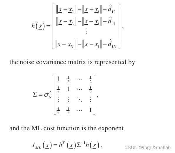
球面散乱数据插值方法/似然估计SI/ML
麦克风阵列声源定位
3.算法具体理论
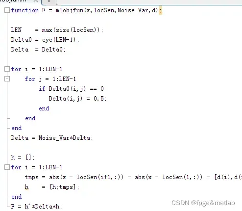
这部分的程序如下:
这部分理论如下所示:
本文的最终算法是:
4.部分核心代码
clc;
clear;
close all;
warning off;
addpath 'func\'
load data\11_11_2KHz24cm_8cmArray.mat
x = data;
figure(1);
plot(x(10000:12000,1),'b-o');hold on;
plot(x(10000:12000,2),'r-o');hold on;
plot(x(10000:12000,3),'k-o');hold on;
plot(x(10000:12000,4),'m-o');hold on;
plot(x(10000:12000,5),'b-s');hold on;
plot(x(10000:12000,6),'r-s');hold on;
plot(x(10000:12000,7),'k-s');hold on;
plot(x(10000:12000,8),'m-s');hold on;
legend('1','2','3','4','5','6','7','8');
[R,C] = size(x);
M = min(R,C); %阵元数目
N = length(x);
x_1 = x(1:N,:);
Delay = zeros(M-1,1);
s_rate = 200000;
Fc = 200e3;
LEN = 2*N-1;%增加精度
CUT = round(0.1*LEN);
%先计算标准值时刻位置
fft_x1 = fft(x_1(:,1),LEN);
fft_x1 = fft(x_1(:,1),LEN);
conj_x1 = conj(fft_x1);
Sxy = fft_x1.*conj_x1;
Cxy = fftshift(ifft(Sxy.*hamming(max(size(Sxy)))));
[Vmx0,location0] = max(abs(Cxy(CUT:end-CUT)));
for i = 1:M-1
fft_x1 = fft(x_1(:,1),LEN);
fft_xi = fft(x_1(:,i+1),LEN);
conj_x1 = conj(fft_x1);
Sxy = fft_xi.*conj_x1;
Cxy = fftshift(ifft(Sxy.*hamming(max(size(Sxy)))));
[Vmx,location] = max(abs(Cxy(CUT:end-CUT)));
%绝对值
d1 = abs(location-location0);
%真实值
d2 = location-location0;
%计算得到采样点间隔
Delay1(i) = d1;
Delay2(i) = d2;
end
%根据间隔,计算时间和距离延迟
times1 = Delay1./Fc;
dist1 = times1*345;
times2 = Delay2./Fc;
dist2 = times2*345;
disp('采样点个数延迟:');
Delay1
Delay2
disp('采样时间延迟:');
times1
times2
disp('采样距离延迟:');
dist1
dist2
save Gcc.mat Delay1 Delay2 times1 times2 dist1 dist2
%**************************************************************************
%**************************************************************************
%**************************************************************************
clear;
xs_src_actual = [0] ;
ys_src_actual = [0.32];
xi = [0 0.08 0.16 0.24 0 0.08 0.16 0.24];
yi = [0 0 0 0 0.08 0.08 0.08 0.08];
%调用前面的延迟估计
load Gcc.mat
%根据路程差计算声源
%number of Monte Carlo runs
nRun = 100;
%uncomment one of them
%turn off ML calculation
bML = 1;
%calculate corresponding range Rs
Rs_actual = sqrt(xs_src_actual.^2 + ys_src_actual.^2);
bearing_actual = [xs_src_actual; ys_src_actual]/Rs_actual;
%number of sensor (>4)
temp = size(xi);
nSen = temp(1,2);
%RD noise (Choose 1)
Noise_Factor = eps; % noise std = Std_Norm * (source distance).
%we expect bigger noise variance for larger distance.
Noise_Var =(Noise_Factor*Rs_actual)^2;
%Functions
%Random Process
for k=1:nRun, % Monte Carlo Simulation
Xi = [xi' yi'];
Di = sqrt((xi-xs_src_actual).^2 + (yi-ys_src_actual).^2);
locSen = [xi' yi'];
%using N sensors
for i=1:nSen-1
d(i,1) = Di(i+1)-Di(1);
%噪声
delta(i,1) = dist1(i);
s(i,:) = [xi(i+1) yi(i+1)];
Alpha_noise= (bearing_actual + randn(2,1)/15);
end
%set to identity matrix for unweighted case
w = eye(nSen-1);
Sw =(s'*w*s)^(-1)*s'*w;
Ps = s*Sw;
Ps_ortho = eye(nSen-1)-Ps;
%SI method
Rs_SI_cal = 0.5*(d'*Ps_ortho*w*Ps_ortho*delta)/(d'*Ps_ortho*w*Ps_ortho*d);
%Calculate Xs for SI method
Xs_row_SI = 0.5*Sw*(2*Rs_SI_cal*d-delta);
Xs_SI(k,:) = [Xs_row_SI.*Alpha_noise]';
Rs_SI(k,:) = sqrt(Xs_SI(k,1)^2 + Xs_SI(k,2)^2);
bearing_SI(k,:) = Xs_SI(k,:)/Rs_SI(k,:);
%Maximum Likelihood Method
if (bML==1)
%As value obtained from SI as starting guess
x0 = Xs_SI(k,:);
%x0 = [0 ys_src_actual 0]; % Starting guess
%LevenbergMarquardt
options = optimset('Algorithm','Levenberg-Marquardt'); %LM
x = lsqnonlin(@mlobjfun,x0,[],[],options,locSen,Noise_Var,d);
Xs_ML(k,:) = x;
Rs_ML(k,:) = sqrt(Xs_ML(k,1)^2+Xs_ML(k,2)^2);
bearing_ML(k,:) = Xs_ML(k,:)/Rs_ML(k,:);
end
%Calculate bias (i.e., errors) for source location, range and bearing
%SI
bias_Xs_SI(k,1) = Xs_SI(k,1) - xs_src_actual;
bias_Xs_SI(k,2) = Xs_SI(k,2) - ys_src_actual;
%ML
if (bML==1)
bias_Xs_ML(k,1) = Xs_ML(k,1)-xs_src_actual;
bias_Xs_ML(k,2) = Xs_ML(k,2)-ys_src_actual;
end
end
clc;
figure;
bias_Rs_SI = Rs_SI-Rs_actual;
bias_bearing_SI = 180/pi*acos(bearing_SI*bearing_actual);
if (bML==1)
bias_Rs_ML=Rs_ML-Rs_actual;
bias_bearing_ML = 180/pi*acos(bearing_ML*bearing_actual);
end
meanxs_SI=mean(bias_Xs_SI(:,1));
meanys_SI=mean(bias_Xs_SI(:,2));
meanrs_SI=mean(bias_Rs_SI);
meanbear_SI=mean(bias_bearing_SI);
vect_mean_SI=[meanxs_SI;meanys_SI;meanrs_SI;meanbear_SI];
%ML
if (bML==1)
meanxs_ML=mean(bias_Xs_ML(:,1));
meanys_ML=mean(bias_Xs_ML(:,2));
meanrs_ML=mean(bias_Rs_ML);
meanbear_ML=mean(bias_bearing_ML);
vect_mean_ML=[meanxs_ML;meanys_ML;meanrs_ML;meanbear_ML];
end
% Calculate Variance = E[(a - mean)^2]
% -----------------------------------------------------
varxs_SI=var(bias_Xs_SI(:,1));
varys_SI=var(bias_Xs_SI(:,2));
varrs_SI=var(bias_Rs_SI);
varbear_SI=var(bias_bearing_SI);
vect_var_SI=[varxs_SI;varys_SI;varrs_SI;varbear_SI];
%ML
if (bML==1)
varxs_ML=var(bias_Xs_ML(:,1));
varys_ML=var(bias_Xs_ML(:,2));
varrs_ML=var(bias_Rs_ML);
varbear_ML=var(bias_bearing_ML);
vect_var_ML=[varxs_ML;varys_ML;varrs_ML;varbear_ML];
end
% Calculate second moment (RMS)= sqrt {E[a^2]} = sqrt {mean^2 + variance}
% -----------------------------------------------------
rmsxs_SI=sqrt(mean(bias_Xs_SI(:,1)).^2+varxs_SI);
rmsys_SI=sqrt(mean(bias_Xs_SI(:,2)).^2+varys_SI);
rmsrs_SI=sqrt(mean(bias_Rs_SI).^2+varrs_SI);
rmsbear_SI=sqrt(mean(bias_bearing_SI).^2+varbear_SI);
vect_rms_SI=[rmsxs_SI;rmsys_SI;rmsrs_SI;rmsbear_SI];
%ML
if (bML==1)
rmsxs_ML=sqrt(mean(bias_Xs_ML(:,1)).^2+varxs_ML);
rmsys_ML=sqrt(mean(bias_Xs_ML(:,2)).^2+varys_ML);
rmsrs_ML=sqrt(mean(bias_Rs_ML).^2+varrs_ML);
rmsbear_ML=sqrt(mean(bias_bearing_ML).^2+varbear_ML);
vect_rms_ML=[rmsxs_ML;rmsys_ML;rmsrs_ML;rmsbear_ML];
end
% Calculate Cramer Rao Bound
%
cov_mat=Noise_Var.*(0.5*ones(length(d))+0.5*eye(length(d)));
for i=1:length(d)
a1=[xs_src_actual-locSen(i+1,1) ys_src_actual-locSen(i+1,2)];
a2=sqrt((xs_src_actual-locSen(i+1,1))^2+(ys_src_actual-locSen(i+1,2))^2);
b1=[xs_src_actual-locSen(1,1) ys_src_actual-locSen(1,2)];
b2=sqrt((xs_src_actual-locSen(1,1))^2+(ys_src_actual-locSen(1,2))^2);
jacobian(i,:)= (a1/a2)-(b1/b2);
end
fisher=jacobian'*inv(cov_mat)*jacobian;
crlb= trace(fisher^-1); % compare with MSE of Rs
% -----------------------------------------------------
% Generate Plots
% -----------------------------------------------------
% hfig1=figure;
if (bML==1)
plot(xi, yi,'bv',Xs_SI(:,1), Xs_SI(:,2),'mo',Xs_ML(:,1), Xs_ML(:,2), 'kd'); % plot both SI and ML
hold on
plot(xs_src_actual, ys_src_actual,'rs','LineWidth',2,'MarkerEdgeColor','k','MarkerFaceColor','g','MarkerSize',6); % plot both SI and ML
else
plot(xi, yi,'bv', xs_src_actual, ys_src_actual, 'r^', Xs_SI(:,1), Xs_SI(:,2), 'mo'); % plot just SI only
end
title('Sensor and Source Location');
str1=sprintf('[Xs, Ys, Zs, Rs, Bearing], Noise Std = %s*Rs',Noise_Factor);
str2=sprintf('SI Method');
str3=sprintf('RMS = [%s, %s, %s, %s, %s]', rmsxs_SI, rmsys_SI,rmsrs_SI, rmsbear_SI);
str4=sprintf('Mean = [%s, %s, %s, %s, %s]', meanxs_SI, meanys_SI,meanrs_SI, meanbear_SI);
str5=sprintf('Variance = [%s, %s, %s, %s, %s]', varxs_SI, varys_SI,varrs_SI, varbear_SI);
if (bML==1)
str6=sprintf('ML Method');
str7=sprintf('RMS = [%s, %s, %s, %s, %s]', rmsxs_ML, rmsys_ML,rmsrs_ML, rmsbear_ML);
str8=sprintf('Mean = [%s, %s, %s, %s, %s]', meanxs_ML, meanys_ML, meanrs_ML, meanbear_ML);
str9=sprintf('Variance = [%s, %s, %s, %s, %s]', varxs_ML, varys_ML, varrs_ML, varbear_ML);
str=sprintf('%s \n%s \n%s \n%s \n%s \n%s \n%s \n%s \n%s', str1, str2, str3, str4,str5, str6, str7, str8, str9);
legend('sensor location', 'calculated source location(SI)','calculated source location (ML)','actual source location ' );
else
str=sprintf('%s \n%s \n%s \n%s \n%s \n%s \n%s \n%s \n%s', str1, str2, str3, str4,str5);
legend('sensor location', 'actual source location', 'calculated source location (SI)');
end
xlabel('Distance (metres) in X direction');
ylabel('Distance (metres) in Y direction');
% generate results output files
fid = fopen('results.txt','w');
for k=1:nRun,
fprintf(fid,'%e\t%e\t%e\t%e\n',bias_Xs_SI(k,1),bias_Xs_SI(k,2), bias_Rs_SI(k), bias_bearing_SI(k));
end
fprintf(fid,'\n%e\t %e\t %e\t %e\t %e\n', meanxs_SI, meanys_SI, meanrs_SI, meanbear_SI);
fprintf(fid,'%e\t %e\t %e\t %e\t %e\n', varxs_SI, varys_SI, varrs_SI, varbear_SI);
fprintf(fid,'%e\t %e\t %e\t %e\t %e\n', rmsxs_SI, rmsys_SI, rmsrs_SI, rmsbear_SI);
fclose(fid);
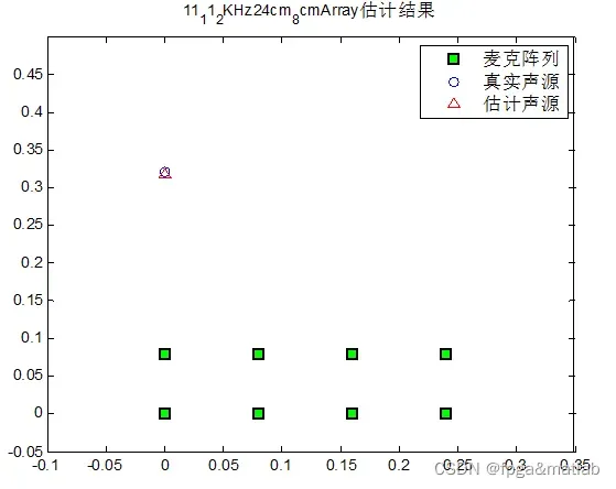
axis([-0.1,0.35,-0.05,0.5]);5.仿真演示
6.本算法写论文思路
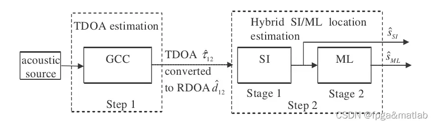
第一部分时间延迟
用8个麦克风阵列采集一组正弦波声源信号. 麦克的位置是已知的. 这样对于同一个声源, 不同麦克采集到的信号会有时延. 以其中的一个声源作为参考用GCC-PHAT方法就可以得到七个time delay. 声音传播速度已知就可以得到七个range difference of arrival
第二部分估计声源位置
用路程差就可以估算声源的位置. 用到两个方法 hybrid spherical interpolation/maximum likelihood (SI/ML) estimation method(应该叫球面散乱数据插值方法/最大似然估计) 然后就可以得到声源坐标, 公式和MATLAB代码文献里都有,
7.参考文献
[1]王丽丽, 徐应祥. 基于散乱数据的球面自然样条插值法[J]. 成都信息工程学院学报, 2012, 27(5):5.
8.相关算法课题及应用
麦克风定位
麦克风阵列
声源定位
A36-04
文章出处登录后可见!
已经登录?立即刷新