前言:本系列文章是关于三维点云处理的常用算法,深入剖析pcl库中相关算法的实现原理,并以非调库的方式实现相应的demo。
1. 最近邻问题概述
(1)最邻近问题:对于点云中的点,怎么去找离它比较近的点
(2)获取邻域点的两种方法:KNN和RNN
-
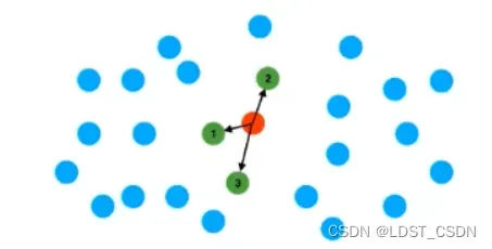
KNN:如图所示,红色点是要查找的点,蓝色点是数据库中的点,图中是找离红色点最近的3个点,显示出来就是图中的绿色点。
-
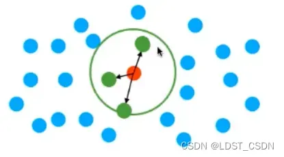
Radius-NN
以上述红色点为圆心,以所选值为半径画圆,圆内的点就是所要找的点
(3)点云最近邻查找的难点 -
点云不规则
-
点云是三维的,比图像高一维,由此造成的数据量是指数上升的。当然,可以建一个三维网格,把点云转化为一个类似于三维图像的东西,但是这也会带来一些矛盾。因为如果网格很多,分辨率足够大,但处理网格需要的内存就很大;如果网格很少,内存够了,但是分辨率又太低。并且,网格中大部分区域都是空白的,所以网格从原理上就不是很高效。
-
点云数据量通常非常大。比如,一个64线的激光雷达,它每秒可产生2.2million个点,如果以20Hz的频率去处理,就意味着每50ms要处理110000个点,如果使用暴力搜索方法对这110000个点都找它最邻近的点,那么计算量为:
(4)最近邻查找:BST、Kd-tree、Octree的共同核心思想 -
空间分割
将空间分割成多个部分,然后在每个小区域中去搜索 -
搜索停止条件
若已知目标点到某一点的距离,那么对于超过这一距离的范围就不需要进行搜索,这个距离也被称为”worst distance”
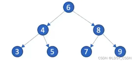
2. 二叉树(Binary Search Tree, BST)
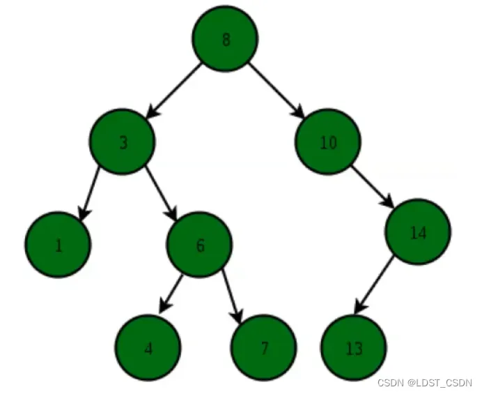
(1)二叉搜索树的特点(一维数据)
- 结点的左子树上的值都小于该根结点的值
- 结点的右子树上的值都大于该根节点的值
- 每一个左右子树都是一个BST
class Node:
    def __init__(self, key, value=-1):
        self.left = None
        self.right = None
        self.key = key
        self.value = value  # 这里的value表示当前点的其他属性,比如颜色、编号等

Data generation ——  随机产生一串数字
    db_size = 10
    data = np.random.permutation(db_size).tolist()

Recursively insert each an element  ——  构造BST的具体实现
def insert(root, key, value=-1):
    if root is None:
        root = Node(key, value)
    else:
        if key < root.key:
            root.left = insert(root.left, key, value)
        elif key > root.key:
            root.right = insert(root.right, key, value)
        else:
            pass
    return root

Insert each element  ——  主函数调用
root = None
for i point in enumerate(data):
    root = insert(root, point, i)  # 这里的value(i)表示的是当前点在原始数组中的位置
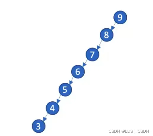
(3)BST的复杂度
- 最坏情况下,二叉树的各结点顺次链接,排成一列,此时复杂度为
,其中
为BST的高度,也是BST中结点个数
- 最好情况下,BST是处于平衡状态的,此时复杂度为
,
为BST中结点总数
# 递归法
def search_recursive(root, key):
    if root is None or root.key == key:
        return root
    if key < root.key:    # 表明key在当前的左子树上
        return search_recursive(root.left, key)
    elif key > root.key: # 表明key在当前的右子树上
        return search_recursive(root.right, key)

# 迭代法  ——  通过栈来实现(不断迭代更新current_node)
def search_iterative(root, key):
    current_node = root
    while current_node is not None:
        if current_node.key == key:
            return current_node
        elif current_node.key < key:
            current_node = current_node.right
        elif current_node.key > key:
            current_node = current_node.left
    return current_node
(5)递归法与迭代法的特点
- 递归
好处:实现简单,容易理解,代码简短
坏处:由于递归需要不停地去压栈,所以每一次递归就是在内存中记录当前递归的位置,因此递归需要的内存空间,这里的
就是递归的次数
- 迭代
优点:它用一个量current_node来表示当前的位置,因此它所需的存储空间为;另外,由于GPU对于堆栈是比较困难的,往往只支持20多层的堆栈,很多时候是不够用的,可能会造成栈溢出(stack-overflow),而且在GPU上实现递归是非常慢的,迭代法可以避免这一问题
缺点:实现起来较为困难
(6)深度优先搜索 (Depth First Traversal)
# 前序遍历  ——  可用于复制一棵树
def preorder(root):
    if root is not None:
        print(root)
        preorder(root.left)
        preorder(root.right)

# 中序遍历  ——  可用于排序
def inorder(root):
    if root is not None:
        inorder(root.left)
        print(root)
        inorder(root.right)

# 后序遍历  ——  可用于删除一个结点
def postorder(root):
    if root is not None:
        postorder(root.left)
        postorder(root.right)
        print(root)
(7)KNN——寻找K个最近邻的点
寻找当前点的K个最近邻点关键在于如何确定worst dist,具体步骤如下:
- 建立一个容器container来存储当前KNN的结果,并将容器中的结果进行排序:例如,当K = 6时,当前KNN结果为[1, 2, 3, 4, 4.5, inf]
- 容器中最后一个就是worst dist,对于新增结点,若新增结点与当前结点计算出来的dist小于当前worst dist,则将其添加到容器中,同时更新worst:例如,若新增结点计算出来的dist为6,则容器中先腾出空间[1, 2, 3, 4, 4.5, 4.5],然后再将当前dist放入到容器中,结果为[1, 2, 3, 4, 4.5, 6],此时worst dist为6
代码实现:构建容器KNNReslutSet
class DistIndex:
    def __init__(self, distance, index):
        self.distance = distance
        self.index = index

    def __lt__(self, other):
        return self.distance < other.distance

class KNNResultSet:
    '''
        用于存储KNN查找结果的容器
        capacity: 容器大小
        count: 当前容器中的元素个数
        worst_dist: 容器结果中的最大值(最长距离)
        dist_index_list: 容器中各个结果距离所对应的结点序号
    '''
    def __init__(self, capacity):
        self.capacity = capacity
        self.count = 0
        self.worst_dist = 1e10  # 初始时,将容器中的数据设置大一些
        self.dist_index_list = []
        for i in range(capacity):
            self.dist_index_list.append(DistIndex(self.worst_dist, 0))
        self.comparison_counter = 0

    def size(self):
        return self.count

    def full(self):
        return self.count == self.capacity

    def worstDist(self):
        return self.worst_dist

    def add_point(self, dist, index):
        self.comparison_counter += 1
        if dist > self.worst_dist:
            return
        if self.count < self.capacity:
            self.count += 1  # 若当前容器元素个数 小于 容器容量,则新增空位

        i = self.count - 1  # 因为是从0开始索引的,故将i定位到新增空位处的索引上
        # 下面其实是将容器中的元素进行排序(包括新腾出来的空位),排序结果根据dist对应的index进行存储
        while i > 0:
            # 若当前容器的最大距离(最后索引) 大于 当前新增距离dist (上面的4.5与6进行比较)
            if self.dist_index_list[i-1].distance > dist:
                # 则将其往后挪一位,使得整体上是从大到小的顺序
                self.dist_index_list[i] = copy.deepcopy(self.dist_index_list[i-1])
                i -= 1
            else:
                break  # 否则,跳出循环,将当前dist放到最后一个元素后面

        self.dist_index_list[i].distance = dist
        self.dist_index_list[i].index = index
        self.worst_dist = self.dist_index_list[self.capacity-1].distance


KNN查找:在当前以Node为根节点(root)的二叉树中,查找离key最近的K个结点,并将其存储于result_set中
def knn_search(root:Node, result_set:KNNResultSet, key):
    if root is None:
        return False

    # 将根节点root与目标节点key进行比较,也就是将当前根节点root放到容器中,这里root.key - key表示dist,root.value表示index
    result_set.add_point(math.fabs(root.key - key), root.value)
    if result_set.worstDist() == 0:  # 若worstDist为0,表示当前根节点root就是所要找到的节点key
        return True
    # 若当前根节点 大于 目标节点
    if root.key >= key:
        # 则在当前根节点的左子树上进行同样的查找操作
        if knn_search(root.left, result_set, key):
            return True
        # 若当前根节点与目标节点的差 小于 最坏距离,那么还可以寻找较大的节点,使其与目标节点的差在最坏距离之内,因此可往当前根节点的右子树上寻找节点
        elif math.fabs(root.key - key) < result_set.worstDist():
            return knn_search(root.right, result_set, key)
        return False
    else:
        # 反之,若当前根节点 小于 目标节点,则在当前根节点的右子树上进行同样的查找操作
        if knn_search(root.right, result_set, key):
            return True
        # 若当前根节点与目标节点的差 小于 最坏距离,那么还可以寻找较小的节点,使其与目标节点的差在最坏距离之内,因此可往当前根节点的左子树上寻找节点
        elif math.fabs(root.key - key) < result_set.worstDist():
            return knn_search(root.left, result_set, key)
        return False
(8)Radius NN查找
Radius NN查找中worstDist是固定的,因此不需要容器存储查找结果,并通过排序维持worstDist,只需将当前节点和目标节点的差与worstDist进行判断,来确定当前节点是否为目标节点的Radius最近点。
# 新增节点
def add_point(self, dist, index):
    self.comparison_counter += 1
    if dist > self.radius:  # 若当前节点计算出的dist大于radius,则退出(不将其加入到最近点范围内)
        return

    # 反之,若当前节点计算出的dist 小于 radius,则将计算出的dist及该节点的索引index存储到最近点范围
    # 同时存储该点的索引index
    self.count += 1
    self.dist_index_list.append(DistIndex(dist, index))

# Radius NN查找
def radius_search(root:Node, result_set:RadiusNNResultSet, key):
    if root is None:
        return False

    # 计算当前根节点root.key与目标节点key的差,判断它是否可以放入容器中result_set
    result_set.add_point(math.fabs(root.key - key), root.value)

    # 同KNN一样,若当前根节点 大于 目标节点
    if root.key >= key:
        # 则在当前根节点的左子树上进行同样的查找操作
        if radius_search(root.left, result_set, key):
            return True
        # 若当前根节点与目标节点的差 小于 最坏距离,那么还可以寻找较大的节点,使其与目标节点的差在最坏距离之内,因此可往当前根节点的右子树上寻找节点
        elif math.fabs(root.key - key) < result_set.worstDist():
            return radius_search(root.right, result_set, key)
        return False
    else:
        # 反之,若当前根节点 小于 目标节点,则在当前根节点的右子树上进行同样的查找操作
        if radius_search(root.right, result_set, key):
            return True
        # 若当前根节点与目标节点的差 小于 最坏距离,那么还可以寻找较小的节点,使其与目标节点的差在最坏距离之内,因此可往当前根节点的左子树上寻找节点
        elif math.fabs(root.key - key) < result_set.worstDist():
            return radius_search(root.left, result_set, key)
        return False
(9)二叉树的应用
二叉树一般是应用在一维数据上,不能将其应用在高维数据上。因为二叉树的查找依赖于左边小、右边大这一特性,对于一维数据来说,这种大和小可以通过直接比较查询点与当前点的大小来获取。而对于高维数据,在某一维度上的大小并不能代表查询点与当前点的大小,故不能应用于高维数据。
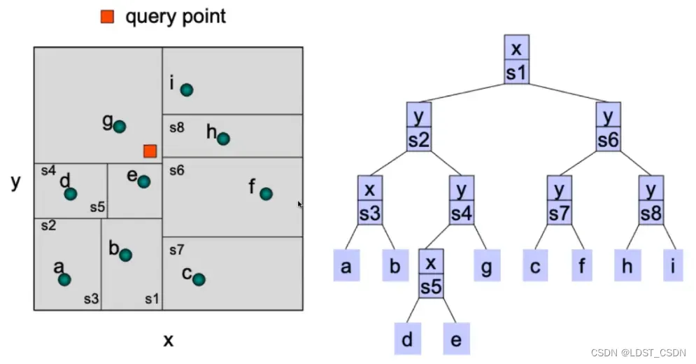
3. Kd-tree
kd-tree通常应用于高维空间(任意维)中,在每个维度上进行一次二叉树,就称为Kd-tree。每次划分时,在每个维度的某一超平面上将样本划分成两部分。另外,通过设置leaf-size来定义停止划分空间的条件,若当前结点个数小于leaf-size,则停止划分。其中,每次划分时的维度可以轮流切换,即x-y-z-x-y-z。
以二维为例,设置leaf-size=1,如下图所示:
class Node:
    def __init__(self, axis, value, left, right, point_indices):
        self.axis = axis  # 当前要切分的维度,比如说接下来是要垂直于哪个轴进行切分
        self.value = value  # 定义当前所要切分维度中的位置,对应上面就是y轴上的位置
        self.left = left  # 定义当前结点的左节点
        self.right = right  # 定义当前结点的右节点
        self.point_indices = point_indices  # 存储属于当前划分区域的结点的序号

    # 若当前结点为一个leaf,则没有必要继续往下划分
    def is_leaf(self):
        # 因为由下面可知,在构建kdtree过程中,value是初始化为None的
        if self.value is None:
            return True
        else:
            return False
(2)构建kd-tree
def kdtree_recursive_build(root, db, point_indices, axis, leaf_size):
    '''
        root: 所创建的kd-tree的根节点
        db: 源数据集
        point_indices: 点的索引
        axis: 所划分的维度
        leaf_size: 最小节点的大小
    '''
    if root is None:  # 若根节点为空,则根据节点的属性创建根节点
        root = Node(axis, None, None, None, point_indices)

    # 若所要划分的样本数量 大于 最小样本数,则进行kd-tree划分,如下:
    if len(point_indices) > leaf_size:
        # 以某一个维度(axis)将db中的点进行排序(这里的排序算法sort_key_by_value是如何得到的?)
        point_indices_sorted, _ = sort_key_by_value(point_indices, db[point_indices, axis])
        # 通过中间靠左位置获取排序后的中间左点(索引及其值)
        middle_left_idx = math.ceil(point_indices_sorted.shape[0] / 2) - 1
        middle_left_point_idx = point_indices_sorted[middle_left_idx]
        middle_left_point_value = db[middle_left_point_idx, axis]

        # 通过中间靠右位置获取排序后的中间右点(索引及其值)
        middle_right_idx = middle_left_idx + 1
        middle_right_point_idx = point_indices_sorted[middle_right_idx]
        middle_right_point_value = db[middle_right_point_idx, axis]

        # 以中间两点的平均值作为根节点值
        root.value = (middle_left_point_value + middle_right_point_value) * 0.5
        # 通过中间左点循环构建左子树
        root.left = kdtree_recursive_build(root.left,
                                           db, 				  															point_indices_sorted[0:middle_right_idx],
                                        axis_round_robin(axis, dim=db.shape[1]),
                                        leaf_size)
        # 通过中间右点循环构建右子树
        root.right = kdtree_recursive_build(root.right,
                                           db, 				  															point_indices_sorted[middle_right_idx:],
                                        axis_round_robin(axis, dim=db.shape[1]),
                                        leaf_size)
        return root

    # 如何选取分割维度:这里采用的是轮换分割,即x-y-x-y
    def axis_round_robin(axis, dim):
    	if axis == dim-1:
	        return 0
    	else:
        	return axis + 1
(3)复杂度
假设建立的kd-tree有个点,并且在每个维度上是均匀平衡的,那么总共有
层,在每一层中进行排序,使得小于的放左边,大于的放右边,这个排序算法的实践复杂度是
,因此,总的时间复杂度是:
。对于空间复杂度,首先,由于每一层中对于每个结点都要存储其index,所以需要
,总的空间复杂度是
。
(4)使用已经构建好的kdtree进行knn查找
关键在于:对于给定查询点query,判断是否要搜索某一区域。若给定的查询点query在某一区域内,或者给定的查询点query到该区域的最小距离 小于 当前的worst dist,那么就需要在这个区域内进行knn查找
def knn_search(root: Node, db: np.ndarray, result_set: KNNResultSet, query: np.ndarray):
    '''
        root: kd-tree的根节点
        db: 源数据集
        result_set: 用于存储knn查找结果的容器,里面维持从小到大的顺序,最后面最大的作为worstDist
        query: 待查询点
    '''
    if root is None:
        return False
    # 判断当前结点是否为叶子节点,若是,则使用暴力查找方法在叶子节点区域中进行查找
    # 因为kd-tree中的叶子节点区域可能不是一个节点,而是多个节点,那么此时就在这多个节点中进行暴力查找
    if root.is_leaf():
        leaf_points = db[root.point_indices, :]
        diff = np.linalg.norm(np.expand_dims(query, 0) - leaf_points, axis=1)
        for i in range(diff.shape[0]):
            result_set.add_point(diff[i], root.point_indices[i])
        return False
    # 若在当前axis维度上,待查询点值小于根节点值,则待查询点在根节点的当前维度的左侧
    if query[root.axis] <= root.value:
        # 则需要在左子树上查找
        knn_search(root.left, db, result_set, query)
        # 另外,右子树上也可能存在离待查询点query较近的点,那么也需要在当前右子树上进行查找。前提是:query在当前维度的值小于根节点的值,且二者之差比最坏距离worstDist小
        ### 这一块还不太懂
        if math.fabs(query[root.axis] - root.value) < result_set.worstDist():
            knn_search(root.right, db, result_set, query)
    else:
        knn_search(root.right, db, result_set, query)
        if math.fabs(query[root.axis] - root.value) < result_set.worstDist():
            knn_search(root.left, db, result_set, query)

    return False
(5)Kd-tree中的Radius NN
同KNN中的Radius NN一样,区别在于此时的worse dist是固定的,而不是在每次分割中需要根据查找点的距离动态更新的。
4. Octree
(1)Octree特点
针对于三维数据,每个维度进行划分,分割一次会得到8个部分。Octree的好处是:高效,不需要经过根节点就可以提前终止划分。因为:若以查询点为中心,以固定值为半径形成一个球,如果这个球完全落在了某个立方体内,那么此时的搜索范围就可以限定在这个小立方体内。而kd-tree中每一层结点只考虑了一个维度,在当前维度下不知道其他维度是如何分割的,所以只有一个维度信息是不足以确定什么时候可以终止搜索。
(2)Octree的关键流程
- 首先,根据所有点的边界确定最大立方体
- 设置停止搜索条件。主要是设置leaf_size(当前区域中点的个数);设置最小区域(此时最小区域中可能有多个点重叠在一起),设置最小区域的初衷是:在某些情况下,某一区域中可能存在重复点,此时不需要划分到每个区域中只包含一个点,将这些重复点划分到一个区域中即可。另外,如果在这种情况下不设置最小区域,那么在leaf_size下,相同点(重叠点)是不会划分开的,此时在划分时可能会陷入死循环
(3)创建Octree
octree中节点的结构——octant
class Octant:
    def __init__(self, children, center, extent, point_indices, is_leaf):
        self.children = children  # 每次划分时的子节点(8个)
        self.center = center      # 中心点
        self.extent = extent      # 半个边长(从中心点到其中一个面的距离)
        self.point_indices = point_indices  # 点的索引
        self.is_leaf = is_leaf    # 是否为叶子节点区域

创建octree
def octree_recursive_build(root, db, center, extent, point_indices, leaf_size, min_extent):
    '''
        root: 要构建的octree的根节点
        db:   源数据样本点
        center: 中心点
        point_indices: 各点的索引
        leaf_size: 叶子节点区域大小(叶子节点区域中节点个数)
        min_extent:  最小区域大小
    '''
    if len(point_indices) == 0:  # 若源数据样本中没有点
        return None  # 则返回一个空的octree

    if root is None:  # 若初始时octree的根节点为空
        # 则根据octant节点的属性,创建初始root节点
        root = Octant([None for i in range(8)], center, extent, point_indices, is_leaf=True)

    # 判断是否需要建立Octree —— 若结点总数小于所设置的min_extent(最小元素个数),就不需要建立
    if len(point_indices) <= leaf_size or extent <= min_extent:
        root.is_leaf = True
    # 否则,进行octree的划分
    else:
        root.is_leaf = False  # 首先,表明当前节点并不是leaf_size
        children_point_indices = [[] for i in range(8)]  # 准备8个子空间
        # 下面是通过for循环将每个点放入到对应的子空间中
        for point_idx in point_indices:
            point_db = db[point_idx]  # 根据索引取出当前点
            morton_code = 0
            # 根据当前点与中心点在3个维度上的比较,将空间划分为8份
            if point_db[0] > center[0]:
                morton_code = morton_code | 1
            if point_db[1] > center[1]:
                morton_code = morton_code | 2
            if point_db[2] > center[2]:
                morton_code = morton_code | 4
            # 将当前点归属到对应的子空间中
            children_point_indices[morton_code].append(point_idx)

            # 创建children
            factor = [-0.5, 0.5]
            for i in range(8):
                # 计算每一个子节点的中心点的3个维度坐标
                child_center_x = center[0] + factor[(i & 1) > 0] * extent
                child_center_y = center[1] + factor[(i & 2) > 0] * extent
                child_center_z = center[2] + factor[(i & 4) > 0] * extent
                # 计算每一个子节点的边长
                child_extent = 0.5 * extent
                # 确定每一个子节点的中心点坐标
                child_center = np.asarray([child_center_x, child_center_y, child_center_z])
                # 根据octant参数,递归创建子octree
                root.children[i] = octree_recursive_build(root.children[i],
                                                          db,
                                                          child_center,
                                                          child_extent,
                                                          children_point_indices[i],
                                                          leaf_size,
                                                          min_extent)
        return root
(4)Octree的KNN查找
def inside(query: np.ndarray, radius: float, octant: Octant):
    """
        功能:判断以待查询点query为球心,radius为半径的球是否在Octant中
        query: 待查询点
        radius: 球半径
        octant: 待比较的子区域
    """
    query_offset = query - octant.center
    query_offset_abs = np.fabs(query_offset)  # 当前待查询点query到octant中心的绝对距离
    possible_space = query_offset_abs + radius  # 上述绝对距离加上半径
    # 比较绝对距离加半径与 octant一半边长的大小 若小于则表示query在octant内,反之则表示query在octant外
    return np.all(possible_space < octant.extent)

def overlaps(query: np.ndarray, radius: float, octant: Octant):
    """
        需要仔细琢磨
        功能:判断一个立方体与一个球是否有交集
        query: 待查询点
        radius: 球半径
        octant: 待比较的子区域
    """
    query_offset = query - octant.center
    query_offset_abs = np.fabs(query_offset)  # 当前待查询点query到octant中心的绝对距离
    max_dist = radius + octant.extent  # 将球半径与当前octant一半边长作为最大距离阈值
    if np.any(query_offset_abs > max_dist):   # case1  判断是否相离
        return False
    if np.sum((query_offset_abs < octant.extent).astype(np.int)) >= 2: # case2 球与面是否相交
        return True
    # case3:比较对角线+球半径 与 octant中心到球心之间的距离,来判断球与立方体角点是否相交
    # 另外,通过max来减少一个维度,使其能够判断球是否与立方体的棱边相交
    x_diff = max(query_offset_abs[0] - octant.extent, 0)
    y_diff = max(query_offset_abs[1] - octant.extent, 0)
    z_diff = max(query_offset_abs[2] - octant.extent, 0)

    return x_diff * x_diff + y_diff * y_diff + z_diff * z_diff < radius * radius

def octree_knn_search(root: Octant, db: np.ndarray, result_set: KNNResultSet, query: np.ndarray):
    """
        root: 创建的octree根节点
        db: 源数据样本点
        result_set: 存储搜索结果的容器
        query: 待查询点
    """
    if root is None:  # 若Octree为空,则直接返回False
        return False
    # 若当前区域为is_leaf,则直接将其中的点与待查询点进行逐个比较————暴力查找
    if root.is_leaf and len(root.point_indices) > 0:
        leaf_points = db[root.point_indices, :]  # 取出叶子节点区域中的全部点
        # 计算待查询点与所有叶子节点之间的距离
        diff = np.linalg.norm(np.expand_dims(query, 0) - leaf_points, axis=1)
        # 根据计算出的距离diff,来判断是否可以将对应的点放入到存储容器result_set中
        for i in range(diff.shape[0]):
            result_set.add_point(diff[i], root.point_indices[i])
        return inside(query, result_set.worstDist(), root)  # 这个inside函数表示的是什么意思
    # 若当前区域不是is_leaf,则要找当前结点下的8个子节点
    # 下面的3个if是找到最有可能包含待查询结点的子节点区域
    morton_code = 0
    if query[0] > root.center[0]:
        morton_code = morton_code | 1
    if query[1] > root.center[1]:
        morton_code = morton_code | 2
    if query[2] > root.center[2]:
        morton_code = morton_code | 4
    # 在找到的子节点区域中继续递归下去找,若能够返回True,则表示在当前子节点区域下找到了
    if octree_knn_search(root.children[morton_code], db, result_set, query):
        return True
    # 若返回的是False,则表示上面那个子节点区域中没有找到,需要继续在其他子节点区域中查找
    for c, child in enumerate(root.children):
        # 遍历到上面已经查找过的子节点区域(morton_code) 或者 遍历到的子节点区域为空时
        # 直接跳过,在下一个子节点区域中进行查找
        if c == morton_code or child is None:
            continue
        # overlaps是判断当前octant 与 以待查询点query为圆心、worstDist为半径的球是否有交集————相离
        # 若没有交点(返回的是False),则跳过当前子区域octant不进行查找
        if False == overlaps(query, result_set.worstDist(), child):
            continue
        # 在剩下的子区域中进行查找
        if octree_knn_search(child, db, result_set, query):
            return True
    # 若以待查询点为圆心、worstDist为半径的球被octant包围了,那么就可提前终止搜索
    # inside():表示一个球是否完全被一个立方体所包围
    return inside(query, result_set.worstDist(), root)
(5)Octree的KNN改进查找
若可判断出以当前查询点query为球心、worseDist为半径的球包含一个子区域,那么就不必在其他子区域中查找,只需在这个被包围的子区域中查找即可
def contains(query: np.ndarray, radius: float, octant: Octant):
    """
        功能:判断以query为球心,radius为半径的球是否包围子区域octant
        query: 待查询点
        radius: 球心
        octant: 子区域
    """
    query_offset = query - octant.center
    query_offset_abs = np.fabs(query_offset)  # 当前待查询点query到octant中心的绝对距离

    # 将绝对距离 + 当前octant一半长度 作为 最大距离阈值,如下图所示
    query_offset_to_farthest_corner = query_offset_abs + octant.extent
    return np.linalg.norm(query_offset_to_farthest_corner) < radius
文章出处登录后可见!