1 线性回归

线性回归(Linear regression)是利用回归方程(函数)对一个或多个自变量(特征值)和因变量(目标值)之间关系进行建模的一种分析方式。

h代表学习算法的解决方案或函数，也称为假设（hypothesis）
h(x)代表预测的值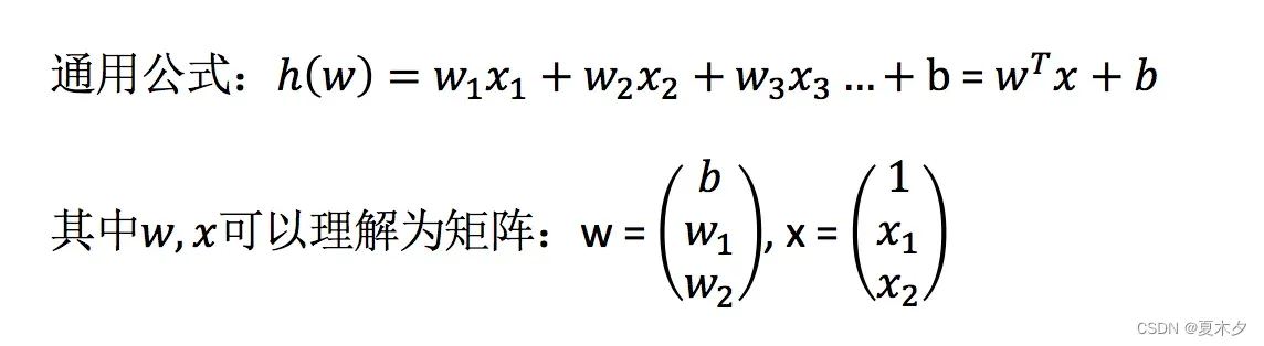

Notice:

只有一个自变量的情况称为单变量回归，多于一个自变量的情况称为多元回归
特征值和目标值之间建立了关系，可以理解为线性模型。
线性回归主要有两种模型，一种是线性关系，一种是非线性关系

2 损失函数

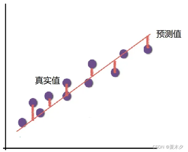
如上图所示，真实结果与我们的预测结果存在一定的误差，这个误差（loss）可以计算出来：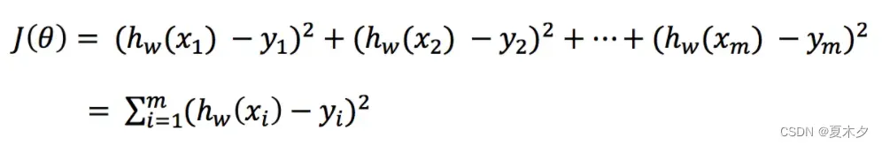

Notice:

yi为第i个训练样本的真实值
h(xi)为第i个训练样本特征值组合预测函数
最小二乘

损失函数（Loss Function）度量单样本预测的错误程度，损失函数值越小，模型就越好。
代价函数（Cost Function）度量全部样本集的平均误差。
目标函数（Object Function）代价函数和正则化函数，最终要优化的函数。

3 优化算法

如何去求模型当中的W，使得损失最小？（目的是找到最小损失对应的W值）

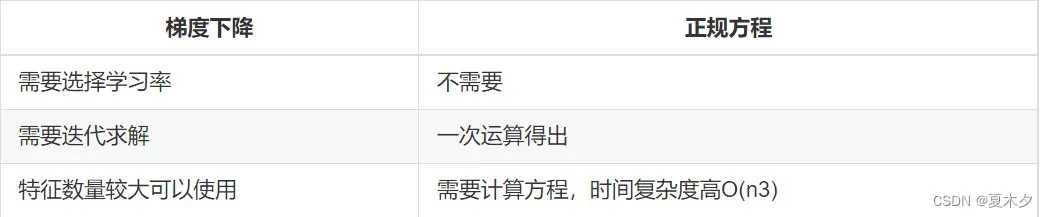
3.1 正规方程

将损失函数转换为矩阵表示法：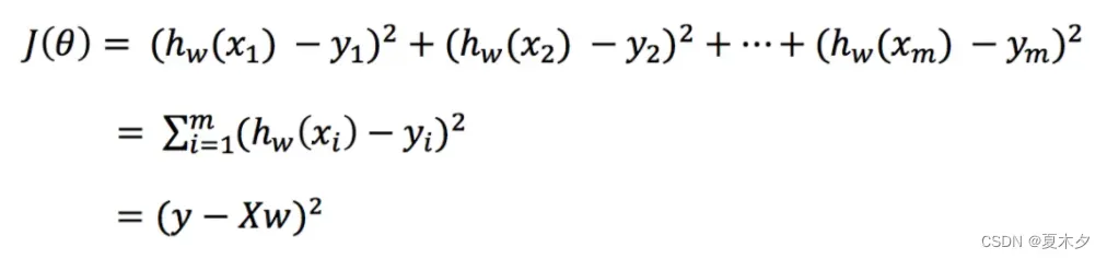

其中y是真实值矩阵，X是特征值矩阵，w是权重矩阵
对其求解关于w（w为自变量）的最小值，导数为零的位置，即为损失的最小值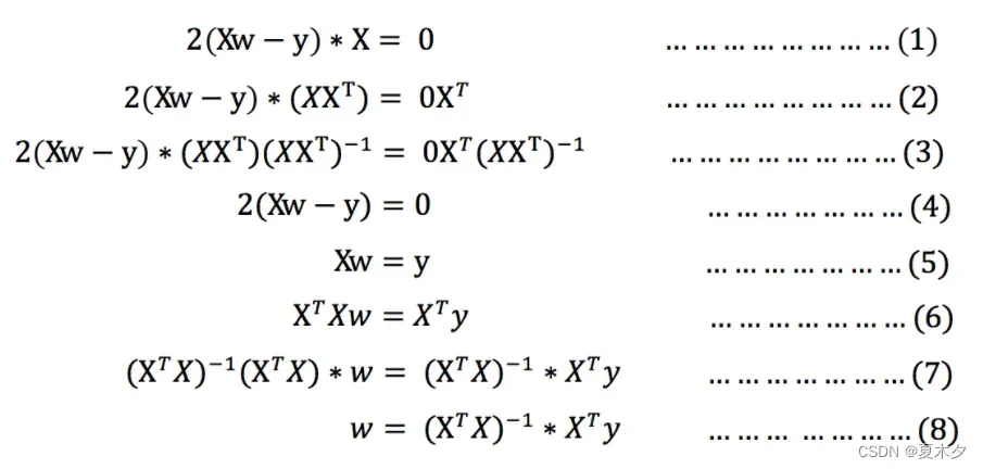

注意：
式(1)到式(2)推导过程中, X是一个m行n列的矩阵，并不能保证其有逆矩阵，但是右乘XT把其变成一个方阵，保证其有逆矩阵。式（5）到式（6）推导过程中，和上类似。

也就是说，正规方程为：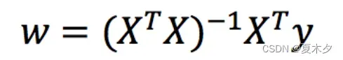

X为特征值矩阵，y为目标值矩阵。直接求到最好的结果
特征太多太复杂时，求解速度太慢，得不到结果

3.2 梯度下降

3.2.1 什么是梯度下降

梯度下降的基本思想可以比作一个下山的过程。

假设一个场景：一个人被困在一座山上，需要从山上下来（找到山的最低点，也就是山谷）。但此时山上的浓雾很浓，能见度很低。因此，下山的路径无法确定，他必须利用周围的信息，寻找下山的路径。这时候，他就可以利用梯度下降算法帮自己下山了。具体来说，就是根据他现在的位置，在这个位置寻找最陡峭的地方，然后朝着山高落下的地方走去。（同理，如果我们的目标是上山，也就是爬到山顶，那么应该是往最陡的方向上去）。然后每走一段距离，就重复使用同样的方法，最后就能顺利到达山谷。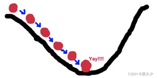

梯度是微积分中一个非常重要的概念

在单变量函数中，梯度实际上是函数的导数，表示函数在给定点的切线斜率。
在多变量函数中，梯度是一个向量，向量是有方向的，梯度的方向指出函数在给定点上升最快的方向，那么梯度的反方向为函数在给定点下降最快的方向。正是我们需要的。所以只要我们一直沿着梯度的反方向行走（原因α为负），我们就可以达到局部最小值！

3.2.2 梯度下降公式

梯度下降公式（Gradient Descent）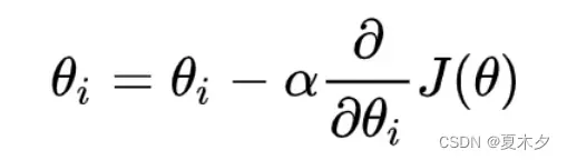

Notice:
α在梯度下降算法中称为学习率或步长，意思是我们可以通过α来控制每一步的距离。 α 不能太大或太小。如果太小，可能会导致延迟和最小步行距离。点太大，会导致漏掉最低点。

因此，使用梯度下降等优化算法，回归具有“自动学习”的能力

3.2.3 梯度下降举例

（1）单变量函数的梯度下降
我们假设有一个单变量的函数 :J(θ) = θ2
函数的微分:J’(θ) = 2θ
初始化，起点为： θº = 1
学习率：α = 0.4
我们开始梯度下降的迭代计算过程：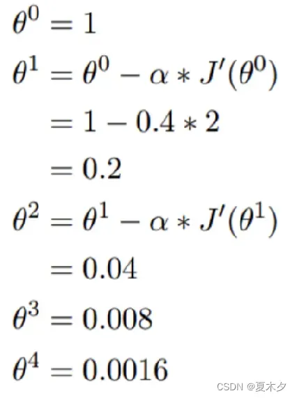

如下图，经过四次操作，也就是四步，基本到了功能的最低点，也就是山脚下。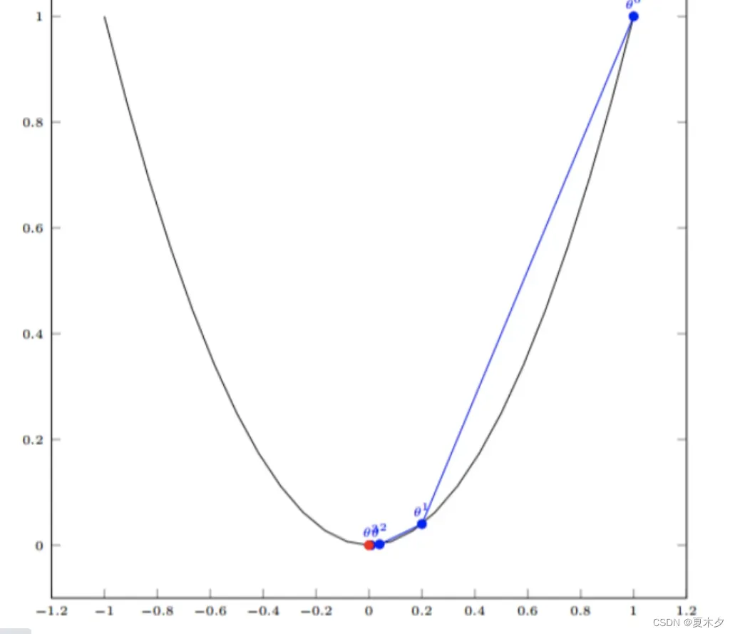

（2）多变量函数的梯度下降

我们假设有一个目标函数：:J(θ) = θ₁² + θ₂²
现在要通过梯度下降法计算这个函数的最小值。我们通过观察就能发现最小值其实就是 (0，0)点。但是接下来，我们会从梯度下降算法开始一步步计算到这个最小值! 我们假设初始的起点为: θº = (1, 3)
初始的学习率为:α = 0.1
函数的梯度为:▽:J(θ) =< 2θ₁ ,2θ₂>
进行多次迭代：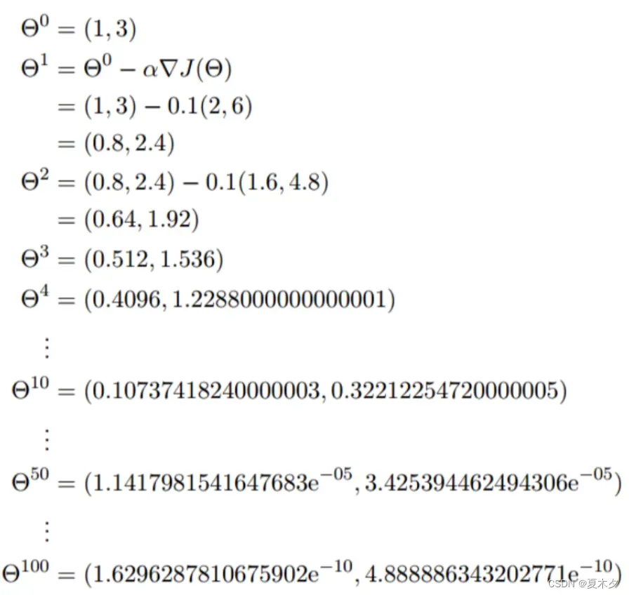

我们发现基本接近函数的最小值点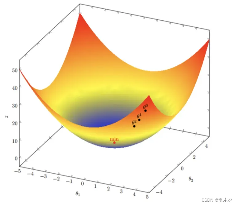

choose:

小规模数据：
– LinearRegression(不能解决拟合问题)
– 岭回归
大规模数据：SGDRegressor

3.2.4 梯度下降算法

常见的梯度下降算法有：

全梯度下降算法(Full gradient descent），
随机梯度下降算法（Stochastic gradient descent），
随机平均梯度下降算法（Stochastic average gradient descent）
小批量梯度下降算法（Mini-batch gradient descent）,

他们都旨在通过计算每个权重的梯度来正确调整权重向量，从而更新权重以尽可能地最小化目标函数。不同之处在于样本的使用方式。
（1）全梯度下降算法（FG）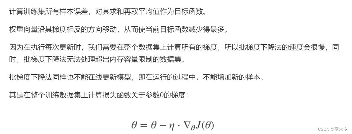

（2）随机梯度下降算法（SG）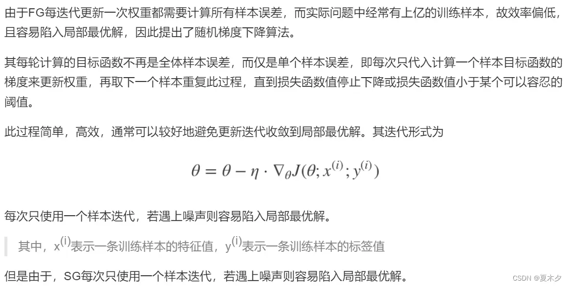

（3）小批量梯度下降算法（mini-bantch）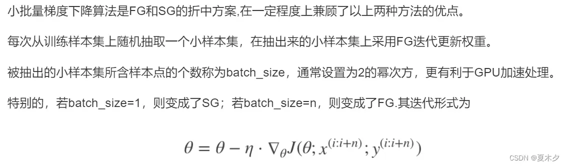

（4）随机平均梯度下降算法（SAG）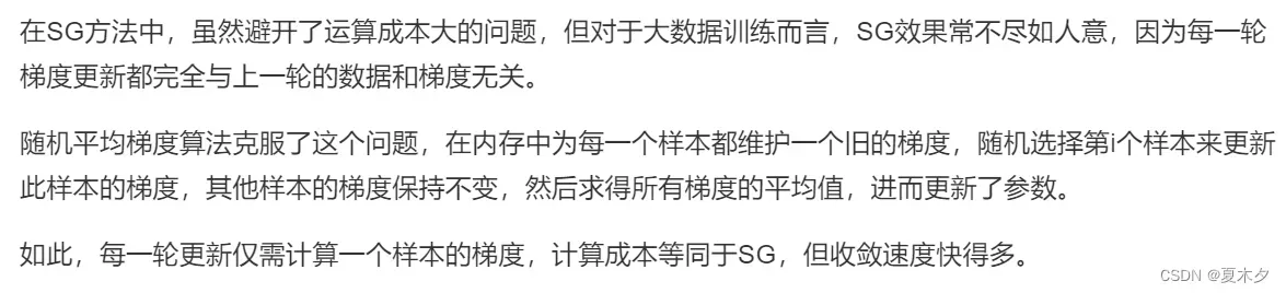

（5）算法比较
以下6幅图反映了模型优化过程中四种梯度算法的性能差异。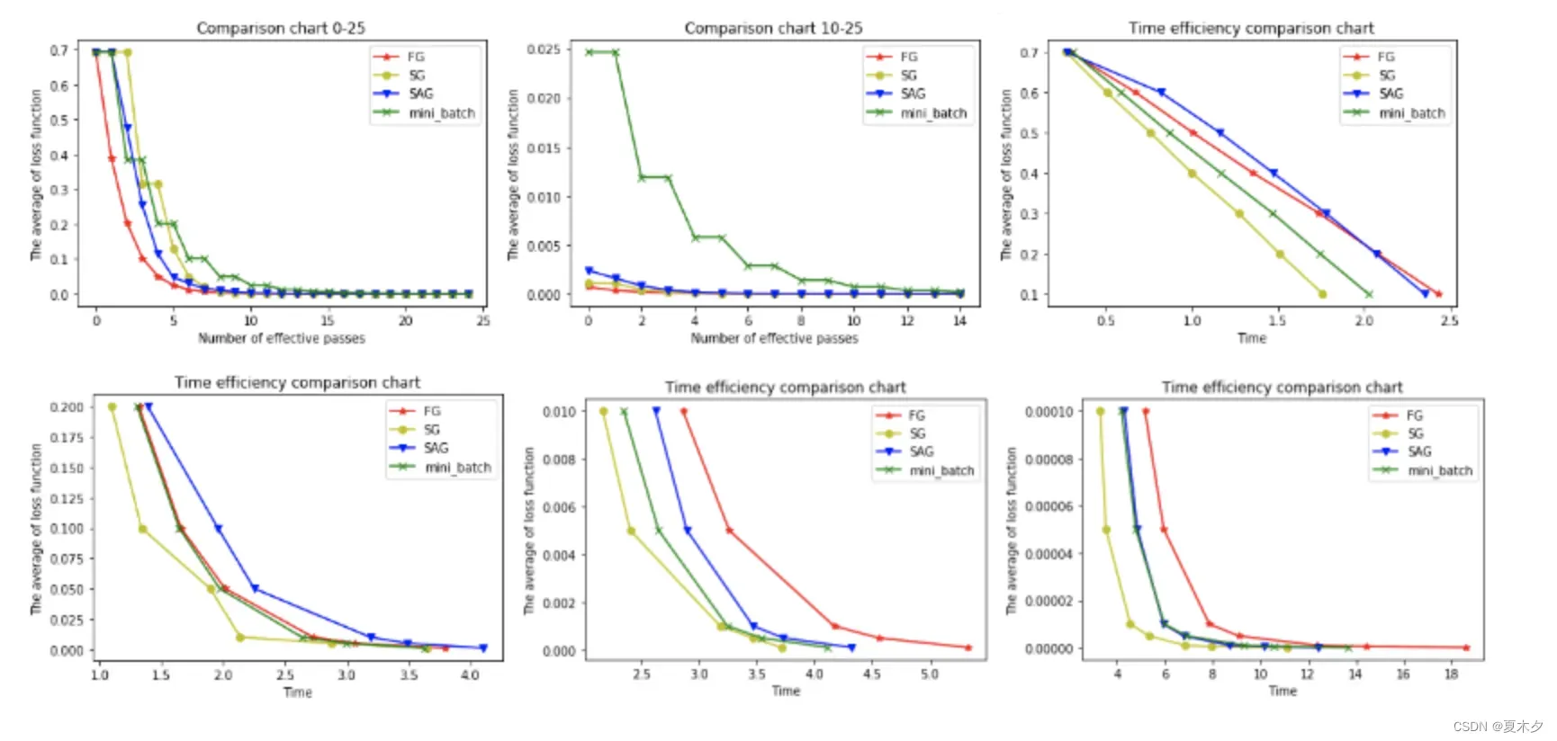

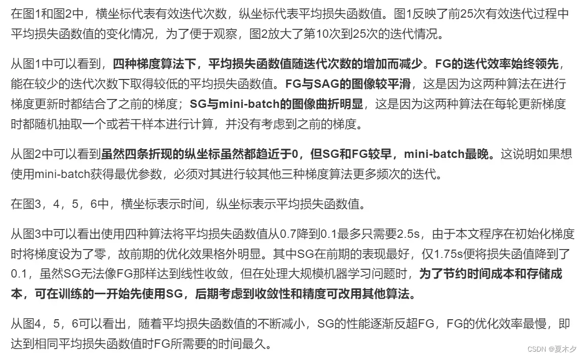
综上所述：

FG方法由于它每轮更新都要使用全体数据集，故花费的时间成本最多，内存存储最大。
SAG在训练初期表现不佳，优化速度较慢。这是因为我们常将初始梯度设为0，而SAG每轮梯度更新都结合了上一轮梯度值。
综合考虑迭代次数和运行时间，SG表现性能都很好，能在训练初期快速摆脱初始梯度值，快速将平均损失函数降到很低。但要注意，在使用SG方法时要慎重选择步长，否则容易错过最优解。
mini-batch结合了SG的“胆大”和FG的“心细”，从6幅图像来看，它的表现也正好居于SG和FG二者之间。在目前的机器学习领域，mini-batch是使用最多的梯度下降算法，正是因为它避开了FG运算效率低成本大和SG收敛效果不稳定的缺点。

3.3 线性回归的使用

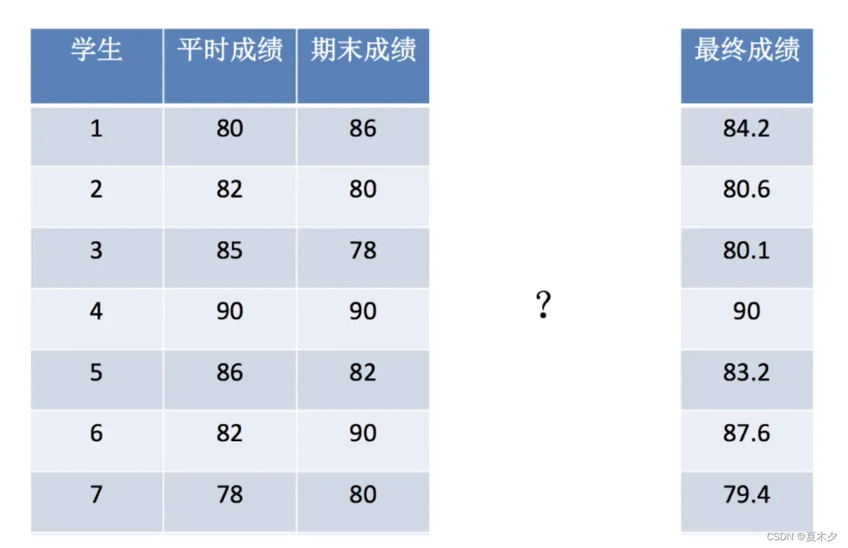
3.3.1 案例1：期末成绩的计算

'''导入模块'''
from sklearn.linear_model import LinearRegression

'''构造数据集'''
x = [[80, 86],
	 [82, 80],
	 [85, 78],
	 [90, 90],
	 [86, 82],
	 [82, 90],
	 [78, 80],
	 [92, 94]]
y = [84.2, 80.6, 80.1, 90, 83.2, 87.6, 79.4, 93.4]

'''模型训练'''
# 实例化一个估计器
estimator = LinearRegression()
# 使用fit方法进行训练
estimator.fit(x,y)
# 查看回归系数值
coef = estimator.coef_
print("系数是：\n",coef) # [0.3 0.7]
# 预测值
prediction = estimator.predict([[100, 80]])
print("预测值是：\n",prediction) # [86.]

3.3.2 案例2：波士顿房价预测

数据集介绍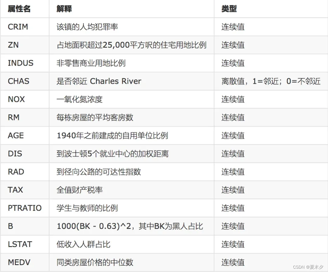

线性回归：正态方程

'''
通过正规方程优化
sklearn.linear_model.LinearRegression(fit_intercept=True)
fit_intercept：是否计算偏置
LinearRegression.coef_：回归系数
LinearRegression.intercept_：偏置
'''
from sklearn.datasets import load_boston
from sklearn.model_selection import train_test_split
from sklearn.preprocessing import StandardScaler
from sklearn.linear_model import LinearRegression
from sklearn.metrics import mean_squared_error

'''获取数据集'''
data = load_boston()

'''划分数据集'''
x_train, x_test, y_train, y_test = train_test_split(data.data, data.target, test_size=0.2)

'''特征工程：数据标准化'''
transfer = StandardScaler()
x_train = transfer.fit_transform(x_train)
x_test = transfer.fit_transform(x_test)

'''机器学习：线性回归（正规方程）'''
estimator = LinearRegression()
estimator.fit(x_train, y_train)

'''模型评估'''
y_predict = estimator.predict(x_test)
print("预测值为：", y_predict)
print("系数值为：", estimator.coef_)
print("偏置值为：", estimator.intercept_)
error = mean_squared_error(y_test, y_predict)
print("均方误差为：", error)

from sklearn.datasets import load_boston
from sklearn.model_selection import train_test_split
from sklearn.preprocessing import StandardScaler
from sklearn.linear_model import LinearRegression
from sklearn.metrics import mean_squared_error

'''获取数据集'''
data = load_boston()

'''划分数据集'''
x_train, x_test, y_train, y_test = train_test_split(data.data, data.target, test_size=0.2)

'''特征工程：数据标准化'''
transfer = StandardScaler()
x_train = transfer.fit_transform(x_train)
x_test = transfer.fit_transform(x_test)

'''机器学习：线性回归（正规方程）'''
estimator = LinearRegression()
estimator.fit(x_train, y_train)

'''模型评估'''
y_predict = estimator.predict(x_test)
print("预测值为：", y_predict)
print("系数值为：", estimator.coef_)
print("偏置值为：", estimator.intercept_)

'''评价'''
error = mean_squared_error(y_test, y_predict) # y_test真实值，y_predict预测值
print("均方误差为：", error)

线性回归：梯度下降

'''
sklearn.linear_model.SGDRegressor(loss="squared_loss", fit_intercept=True, learning_rate ='invscaling', eta0=0.01)
SGDRegressor类实现了随机梯度下降学习，它支持不同的loss函数和正则化惩罚项来拟合线性回归模型。
loss:损失类型
loss=”squared_loss”: 普通最小二乘法
fit_intercept：是否计算偏置
learning_rate : string, optional
学习率填充
'constant': eta = eta0 对于一个常数值的学习率来说，可以使用learning_rate=’constant’ ，并使用eta0来指定学习率。
'optimal': eta = 1.0 / (alpha * (t + t0)) [default]
'invscaling': eta = eta0 / pow(t, power_t)
SGDRegressor.coef_：回归系数
SGDRegressor.intercept_：偏置
'''
from sklearn.datasets import load_boston
from sklearn.model_selection import train_test_split
from sklearn.preprocessing import StandardScaler
from sklearn.linear_model import LinearRegression
from sklearn.metrics import mean_squared_error

'''获取数据集'''
data = load_boston()

'''划分数据集'''
x_train, x_test, y_train, y_test = train_test_split(data.data, data.target, test_size=0.2)

'''特征工程：数据标准化'''
transfer = StandardScaler()
x_train = transfer.fit_transform(x_train)
x_test = transfer.fit_transform(x_test)

'''机器学习-线性回归(特征方程)'''
estimator = SGDRegressor(max_iter=1000)
estimator.fit(x_train, y_train)

'''模型评估'''
y_predict = estimator.predict(x_test)
print("预测值为:\n", y_predict)
print("模型中的系数为:\n", estimator.coef_)
print("模型中的偏置为:\n", estimator.intercept_)

'''评价'''
error = mean_squared_error(y_test, y_predict)
print("误差为:\n", error)

4 欠拟合与过拟合

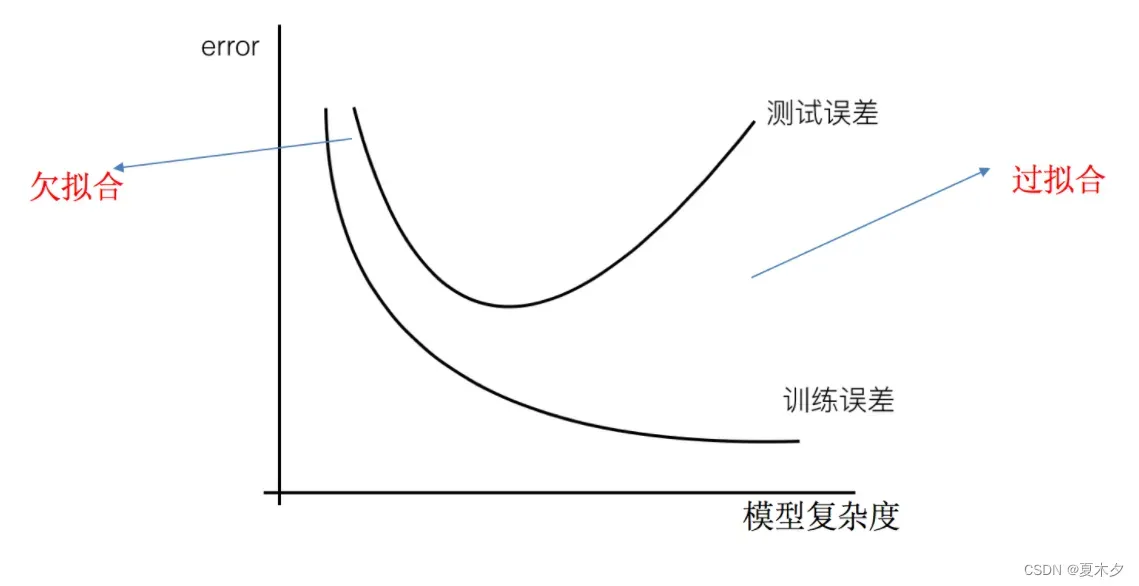
4.1 欠拟合

概念：假设不能更好地拟合训练数据，也不能很好地拟合测试数据集。此时，该假设被认为是欠拟合的。（模型太简单了）

原因：学习数据的特征太少

Solution:

添加其他功能
添加多项式特征

4.2 过拟合

概念：假设可以更好地拟合训练数据，但不能很好地拟合测试数据集。此时，该假设被认为是过拟合的。（模型太复杂）

原因：原始特征太多，有一些噪声特征，模型太复杂，因为模型试图考虑到每个测试数据点

Solution:

重新清理数据
增加训练数据量
Regularization
降低特征维度，防止维度灾难

Regularization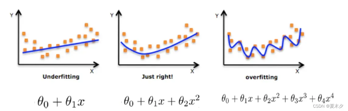

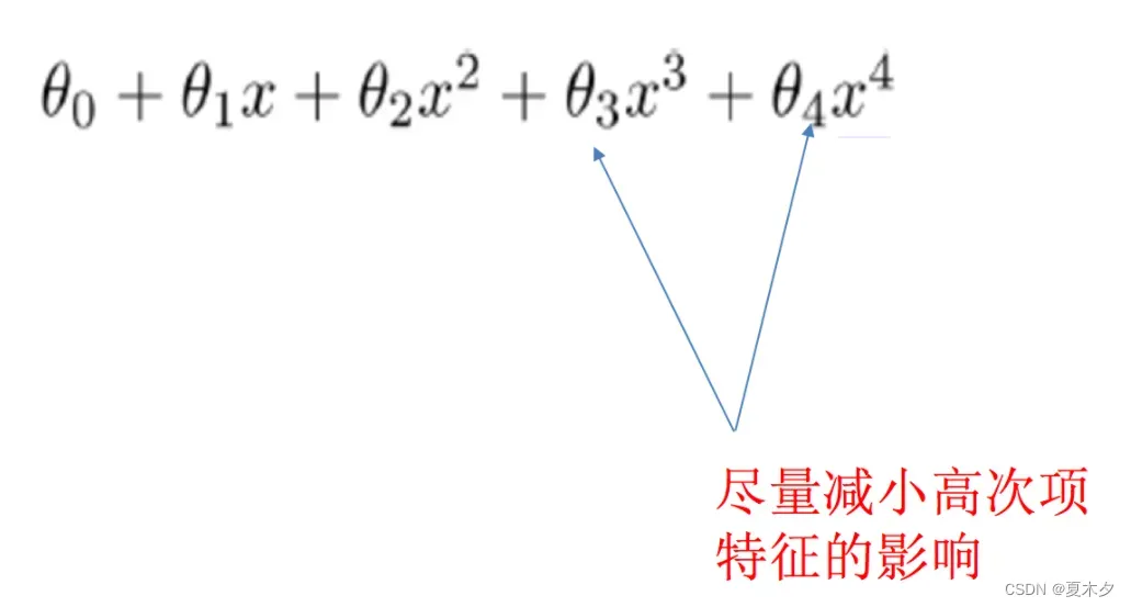
在学习过程中，数据提供的特征可能会影响模型的复杂度或者这个特征的数据点异常大，所以算法在学习的时候尽量减少这个特征的影响（甚至删除某个特征的影响），这是正则化。

L1正则化

作用：可以使得其中一些W的值直接为0，删除这个特征的影响
LASSO回归

L2正则化

作用：可以使得其中一些W的都很小，都接近于0，削弱某个特征的影响
优点：参数越小，模型越简单，模型越简单，越不容易造成过拟合。
Ridge回归

次元灾难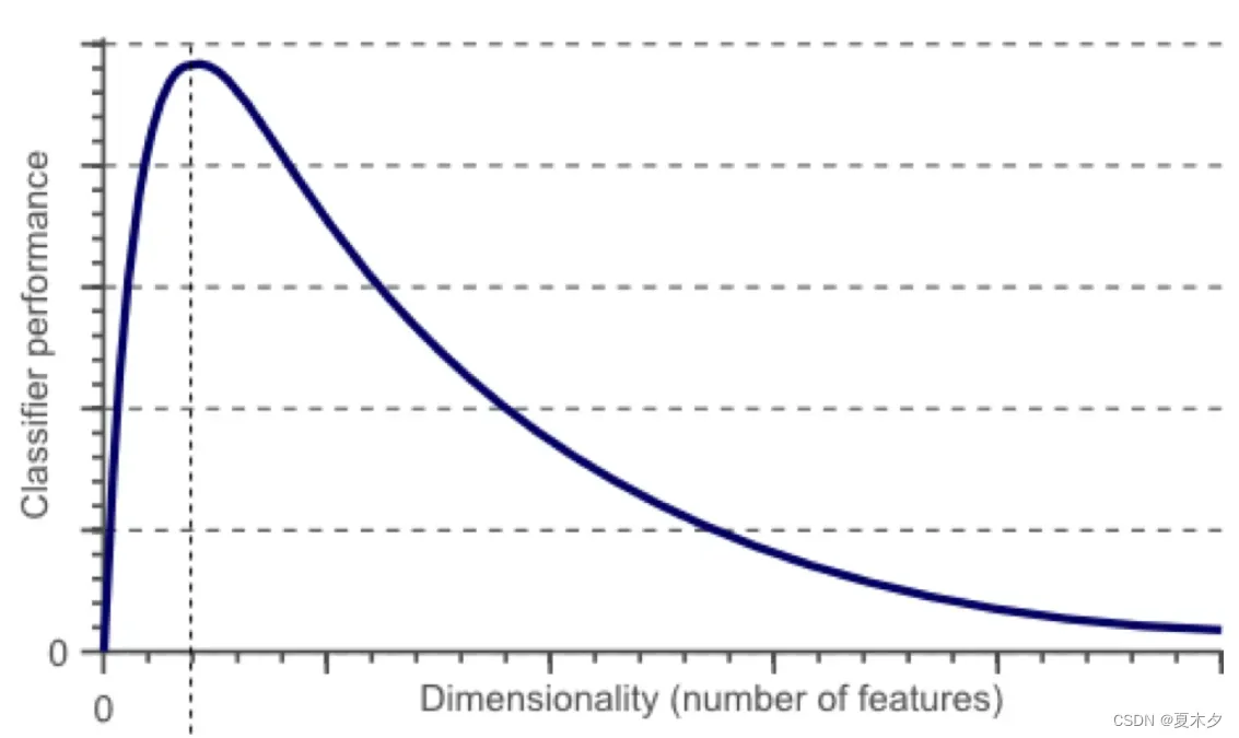

随着维度的增加，分类器的性能逐渐提高，达到一定点后，其性能逐渐下降。

5 正则化线性模型

5.1 Ridge Regression 岭回归

岭回归是线性回归的正则化版本，即在原来的线性回归的 cost function 中添加正则项：
为了达到在拟合数据的同时使模型权重尽可能小的目的，岭回归代价函数：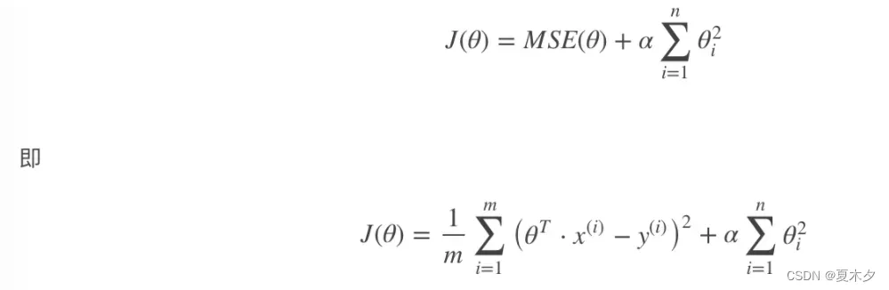

Notice:
α=0时，岭回归退化为线性回归

from sklearn.datasets import load_boston
from sklearn.model_selection import train_test_split
from sklearn.preprocessing import StandardScaler
from sklearn.linear_model import Ridge, RidgeCV
from sklearn.metrics import mean_squared_error
import joblib

'''获取数据集'''
data = load_boston()

'''划分数据集'''
x_train, x_test, y_train, y_test = train_test_split(data.data, data.target, test_size=0.2)

'''特征工程：数据标准化'''
transfer = StandardScaler()
x_train = transfer.fit_transform(x_train)
x_test = transfer.fit_transform(x_test)

'''机器学习：岭回归
sklearn.linear_model.Ridge(alpha=1.0, fit_intercept=True,solver="auto", normalize=False)
具有l2正则化的线性回归
- alpha:正则化力度，也叫 λ，λ取值：0~1 1~10（正则化力度越大，权重系数越小，反之，越大）
- solver:会根据数据自动选择优化方法，sag:如果数据集、特征都比较大，选择该随机梯度下降优化
- normalize:数据是否进行标准化，normalize=False:可以在fit之前调用preprocessing.StandardScaler标准化数据
Ridge.coef_:回归权重
Ridge.intercept_:回归偏置
'''
# estimator = Ridge()
# estimator = RidgeCV(alphas=(0.1, 1, 10))
# estimator.fit(x_train, y_train)

'''模型的保存与加载
import joblib
保存：joblib.dump(estimator, 'test.pkl')
加载：estimator = joblib.load('test.pkl')
'''
# joblib.dump(estimator, 'test.pkl')
estimator = joblib.load('test.pkl')

'''模型评估'''
y_predict = estimator.predict(x_test)
print("预测值为：", y_predict)
print("系数值为：", estimator.coef_)
print("偏置值为：", estimator.intercept_)
error = mean_squared_error(y_test, y_predict)
print("均方误差为：", error)

5.2 Lasso 回归

Lasso回归的代价函数：
Lasso Regression 的代价函数在 θi=0处不可导，可以在θi=0处用一个次梯度向量(subgradient vector)代替梯度：

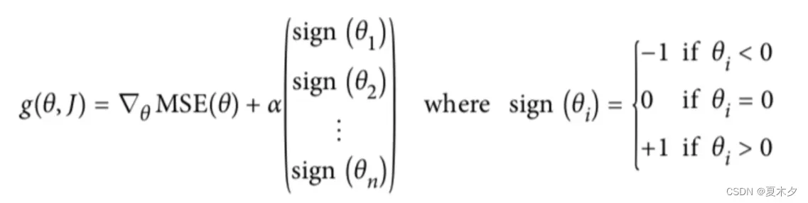
Notice:

Lasso Regression 的代价函数在 θi=0处是不可导的
倾向于完全消除不重要的权重

5.3 Elastic Net 弹性网络

弹性网络的成本函数：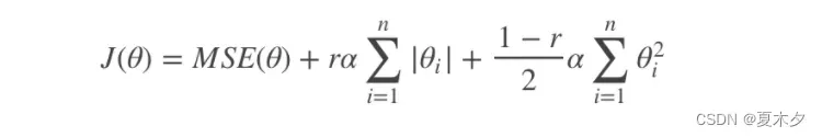

弹性网络在岭回归和Lasso回归中进行了折中，通过混合比(mix ratio) r 进行控制：

r=0：弹性网络变为岭回归
r=1：弹性网络便为Lasso回归

Notice:
summary:

常用：岭回归
假设只有几个功能有用：
– 弹性网络
– Lasso
– 一般来说，弹性网络的使用更为广泛。因为在特征维度高于训练样本数，或者特征是强相关的情况下，Lasso回归的表现不太稳定。

5.4 Early stopping

Early Stopping 也是正则化迭代学习的方法之一。
该方法是在验证错误率达到最小值时停止训练。

文章出处登录后可见！

已经登录？立即刷新

线性回归算法