paper：PaDiM: a Patch Distribution Modeling Framework for Anomaly Detection and Localization

code1：https://github.com/xiahaifeng1995/PaDiM-Anomaly-Detection-Localization-master 

code2：https://github.com/openvinotoolkit/anomalib 

背景

异常检测是一个区分正常类别与异常类别的二分类问题，但实际应用中我们经常缺乏异常样本，并且异常可能会有意想不到的模式，所以训练一个全监督的模型是不切实际的。因此，异常检测模型通常以单类别学习的模式，即训练集中只包含正常样本，在测试阶段，与正常类别不同的样本被归类为异常样本。 

论文的出发点

目前的单类别学习模式的异常检测模型要么需要训练深度神经网络，非常麻烦。要么测试阶段在整个训练集上使用K最近邻算法，KNN算法线性复杂度的特点导致随着训练集的增大，其时间和空间复杂度也随之增大。这两类问题可能会阻碍异常检测算法在工业环境中的部署。针对上述两个问题，本文提出了一个新的异常检测和定位方法PaDiM（Patch Distribution Modeling）。

论文的创新点

PaDiM利用预训练好的CNN进行embedding提取，并且具有以下两个特点：（1）每个patch位置都用一个多元高斯分布来描述。（2）PaDiM考虑到了CNN不同语义level之间的关联。此外，在测试阶段，它的时间和空间复杂度都比较小，且独立于训练集的大小，这非常有利于工业部署应用。对于异常检测和定位任务，在MVTec AD和ShanghaiTec Campus两个数据集上，PaDiM超越了现有SOTA方法（2020年本文提出时）。

实现细节

这里以在ImageNet数据集上预训练的resnet18为例讲解下具体实现过程，数据采用mvtec中的bottle类别，共有209张训练图片。

A. Embedding extraction

如上图中间所示，将预训练模型中三个不同层的feature map对应位置进行拼接得到embedding vector，这里分别取resnet18中layer1、layer2、layer3的最后一层，模型输入大小为224×224，这三层对应输出维度分别为(209,64,56,56)、(209,128,28,28)、(209,256,14,14)，这里实现1中是通过将小特征图每个位置复制多份得到与大特征图同样的spatial size，然后再进行拼接。比如28×28的特征图中一个1×1的patch与56×56的特征图中对应位置的2×2的patch相对应，将该1×1的patch复制4份得到2×2大小patch后再与56×56对应位置的2×2 patch进行拼接，下面的代码是通过F.unfold实现的，F.unfold的具体用法见 torch.nn.functional.unfold 用法解读_00000cj的博客-CSDN博客 

def embedding_concat(x, y):
    B, C1, H1, W1 = x.size()  # (209,64,56,56)
    _, C2, H2, W2 = y.size()  # (209,128,28,28)
    s = int(H1 / H2)  # 2
    x = F.unfold(x, kernel_size=s, dilation=1, stride=s)  # (209,256,784)
    x = x.view(B, C1, -1, H2, W2)  # (209,64,4,28,28)
    z = torch.zeros(B, C1 + C2, x.size(2), H2, W2)  # (209,192,4,28,28)
    for i in range(x.size(2)):
        z[:, :, i, :, :] = torch.cat((x[:, :, i, :, :], y), 1)
    z = z.view(B, -1, H2 * W2)  # (209,768,784)
    z = F.fold(z, kernel_size=s, output_size=(H1, W1), stride=s)  # (209,192,56,56)

    return z

实现2中则是通过插值的方法，通过最近邻插值算法将小特征图进行上采样后再与大特征图进行拼接，如下所示，其中因为实现2的输入大小是256×256，因此最大特征图size为64×64

embeddings = features[self.layers[0]]
for layer in self.layers[1:]:
    layer_embedding = features[layer]
    layer_embedding = F.interpolate(layer_embedding, size=embeddings.shape[-2:], mode="nearest")
    embeddings = torch.cat((embeddings, layer_embedding), 1)  # torch.Size([32, 448, 64, 64])

将三个不同语义层的特征图进行拼接后得到(209, 448, 56, 56)大小的patch嵌入向量可能带有冗余信息，因此作者对其进行了降维，作者发现随机挑选某些维度的特征比PCA更有效，在保持sota性能的前提下降低了训练和测试的复杂度，文中维度选择100，因此输出为(209, 100, 56, 56)。

B. Learning of nomality

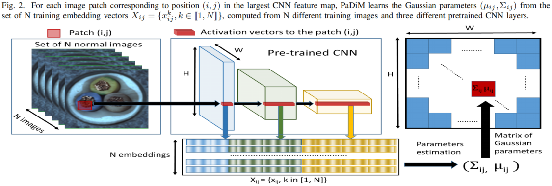
为了学习正常图像在位置 \((i,j)\) 处的特征，我们首先计算 \(N\) 张正常训练图片在位置 \((i,j)\) 处的嵌入向量集和 \(X_{ij}=\left \{ x_{ij}^{k},k\in\left [ 1,N \right ]  \right \}  \)，为了整合这个set的信息假设 \(X_{ij}\) 是通过多元高斯分布 \(\mathcal N(\mu_{ij},{\textstyle \sum_{ij}^{}}  )\) 得到的，其中 \(\mu_{ij}\) 是 \(X_{ij}\) 的样本均值，样本协方差 \({\textstyle \sum_{ij}^{}} \) 通过下式估计得到

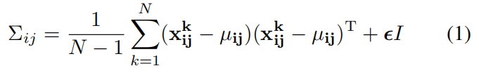
其中正则项 \(\epsilon I\) 保证协方差矩阵时满秩且可逆的，如上图右所示，图像中每个位置都通过高斯参数矩阵与一个多元高斯分别相关联。

实现1是通过numpy中的np.conv函数直接计算协方差矩阵的，代码如下

# randomly select d dimension
embedding_vectors = torch.index_select(embedding_vectors, 1, idx)  # (209,448,56,56) -> (209,100,56,56)
# calculate multivariate Gaussian distribution
B, C, H, W = embedding_vectors.size()
embedding_vectors = embedding_vectors.view(B, C, H * W)  # (209,100,3136)
mean = torch.mean(embedding_vectors, dim=0).numpy()  # (100,3136)
cov = torch.zeros(C, C, H * W).numpy()  # (100,100,3136)
I = np.identity(C)
for i in range(H * W):
    cov[:, :, i] = np.cov(embedding_vectors[:, :, i].numpy(), rowvar=False) + 0.01 * I
# save learned distribution
train_outputs = [mean, cov]
with open(train_feature_filepath, 'wb') as f:
    pickle.dump(train_outputs, f)

实现2则是按式(1)一步步计算得到的协方差矩阵

class MultiVariateGaussian(nn.Module):
    """Multi Variate Gaussian Distribution."""

    def __init__(self, n_features, n_patches):
        super().__init__()

        self.register_buffer("mean", torch.zeros(n_features, n_patches))
        self.register_buffer("inv_covariance", torch.eye(n_features).unsqueeze(0).repeat(n_patches, 1, 1))

        self.mean: Tensor
        self.inv_covariance: Tensor

    @staticmethod
    def _cov(
        observations: Tensor,  # (batch_size, 100), (209,100)
        rowvar: bool = False,
        bias: bool = False,
        ddof: Optional[int] = None,
        aweights: Tensor = None,
    ) -> Tensor:
        """Estimates covariance matrix like numpy.cov.

        Args:
            observations (Tensor): A 1-D or 2-D array containing multiple variables and observations.
                 Each row of `m` represents a variable, and each column a single
                 observation of all those variables. Also see `rowvar` below.
            rowvar (bool): If `rowvar` is True (default), then each row represents a
                variable, with observations in the columns. Otherwise, the relationship
                is transposed: each column represents a variable, while the rows
                contain observations. Defaults to False.
            bias (bool): Default normalization (False) is by ``(N - 1)``, where ``N`` is the
                number of observations given (unbiased estimate). If `bias` is True,
                then normalization is by ``N``. These values can be overridden by using
                the keyword ``ddof`` in numpy versions >= 1.5. Defaults to False
            ddof (Optional, int): If not ``None`` the default value implied by `bias` is overridden.
                Note that ``ddof=1`` will return the unbiased estimate, even if both
                `fweights` and `aweights` are specified, and ``ddof=0`` will return
                the simple average. See the notes for the details. The default value
                is ``None``.
            aweights (Tensor): 1-D array of observation vector weights. These relative weights are
                typically large for observations considered "important" and smaller for
                observations considered less "important". If ``ddof=0`` the array of
                weights can be used to assign probabilities to observation vectors. (Default value = None)


        Returns:
          The covariance matrix of the variables.
        """
        # ensure at least 2D
        if observations.dim() == 1:
            observations = observations.view(-1, 1)

        # treat each column as a data point, each row as a variable
        if rowvar and observations.shape[0] != 1:
            observations = observations.t()

        if ddof is None:
            if bias == 0:
                ddof = 1
            else:
                ddof = 0

        weights = aweights
        weights_sum: Any

        if weights is not None:
            if not torch.is_tensor(weights):
                weights = torch.tensor(weights, dtype=torch.float)  # pylint: disable=not-callable
            weights_sum = torch.sum(weights)
            avg = torch.sum(observations * (weights / weights_sum)[:, None], 0)
        else:
            avg = torch.mean(observations, 0)  # torch.Size([100])

        # Determine the normalization
        if weights is None:
            fact = observations.shape[0] - ddof  # batch_size-1 (209-1)
        elif ddof == 0:
            fact = weights_sum
        elif aweights is None:
            fact = weights_sum - ddof
        else:
            fact = weights_sum - ddof * torch.sum(weights * weights) / weights_sum

        observations_m = observations.sub(avg.expand_as(observations))  # (209,100)

        if weights is None:
            x_transposed = observations_m.t()  # (100,209)
        else:
            x_transposed = torch.mm(torch.diag(weights), observations_m).t()
        covariance = torch.mm(x_transposed, observations_m)  # (100, 100)
        covariance = covariance / fact

        return covariance.squeeze()

    def forward(self, embedding: Tensor) -> List[Tensor]:
        """Calculate multivariate Gaussian distribution.

        Args:
          embedding (Tensor): CNN features whose dimensionality is reduced via either random sampling or PCA.

        Returns:
          mean and inverse covariance of the multi-variate gaussian distribution that fits the features.
        """
        device = embedding.device

        batch, channel, height, width = embedding.size()
        # 训练时batch_size=32,每10个epoch测试一次，因此这里的batch应该是320,但训练集总共只有209张图片，因此这里batch=209
        embedding_vectors = embedding.view(batch, channel, height * width)
        self.mean = torch.mean(embedding_vectors, dim=0)  # (100, 4096)
        covariance = torch.zeros(size=(channel, channel, height * width), device=device)
        identity = torch.eye(channel).to(device)
        for i in range(height * width):
            covariance[:, :, i] = self._cov(embedding_vectors[:, :, i], rowvar=False) + 0.01 * identity

        # calculate inverse covariance as we need only the inverse
        self.inv_covariance = torch.linalg.inv(covariance.permute(2, 0, 1))

        return [self.mean, self.inv_covariance]

    def fit(self, embedding: Tensor) -> List[Tensor]:
        """Fit multi-variate gaussian distribution to the input embedding.

        Args:
            embedding (Tensor): Embedding vector extracted from CNN.

        Returns:
            Mean and the covariance of the embedding.
        """
        return self.forward(embedding)

C. Inference: computation of the anomaly map

文中使用马氏距离 \(M(x_{ij})\) 来计算测试图片在位置 \((i,j)\) 处的异常分数，\(M(x_{ij})\) 表示测试图片的嵌入向量 \(x_{ij}\) 和学习到的分布 \(\mathcal N(\mu_{ij},{\textstyle \sum_{ij}^{}}  )\) 之间的距离，计算方式如下

实现1中直接调用scipy库中的mahalanobis函数来计算马氏距离，代码如下

from scipy.spatial.distance import mahalanobis
# randomly select d dimension
embedding_vectors = torch.index_select(embedding_vectors, 1, idx)

# calculate distance matrix
B, C, H, W = embedding_vectors.size()  # (83,100,56,56)
embedding_vectors = embedding_vectors.view(B, C, H * W).numpy()  # (83,100,3136)
dist_list = []
for i in range(H * W):
    mean = train_outputs[0][:, i]  # (100,)
    conv_inv = np.linalg.inv(train_outputs[1][:, :, i])  # (100,100)
    dist = [mahalanobis(sample[:, i], mean, conv_inv) for sample in embedding_vectors]
    dist_list.append(dist)

测试集一共83张图片，在得到每个像素点的马氏距离后，进行上采样、高斯滤波、归一化的后处理后，就得到了最终的输出，大小和输入相同，维度为 (83, 224, 224)，其中每个位置的值为该像素点为异常类的得分。

from scipy.ndimage import gaussian_filter
dist_list = np.array(dist_list).transpose(1, 0).reshape(B, H, W)  # (3136,83)->(83,3136)->(83,56,56)

# upsample
dist_list = torch.tensor(dist_list)
score_map = F.interpolate(dist_list.unsqueeze(1), size=x.size(2), mode='bilinear',
                          align_corners=False).squeeze().numpy()  # (83,224,224)

# apply gaussian smoothing on the score map
for i in range(score_map.shape[0]):
    score_map[i] = gaussian_filter(score_map[i], sigma=4)

# Normalization
max_score = score_map.max()
min_score = score_map.min()
scores = (score_map - min_score) / (max_score - min_score)  # (83,224,224)

实验

消融实验 

Inter-layer correlation

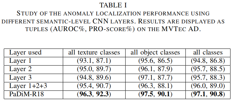
高斯分布和马氏距离在之前已经被用于缺陷检测中了，但没有像PaDiM一样考虑到CNN中不同语义层级之间的关联，作者通过实验对比了单独采用layer1、2、3，将单独采用单层特征的三个模型相加进行模型融合，以及本文的方法。通过上表可以看出，模型融合比采用单层特征的单个模型效果更好，但这并没有考虑到三层之间的关联，PaDiM考虑到了这点并获得了最优的结果。 

Dimensionality reduction

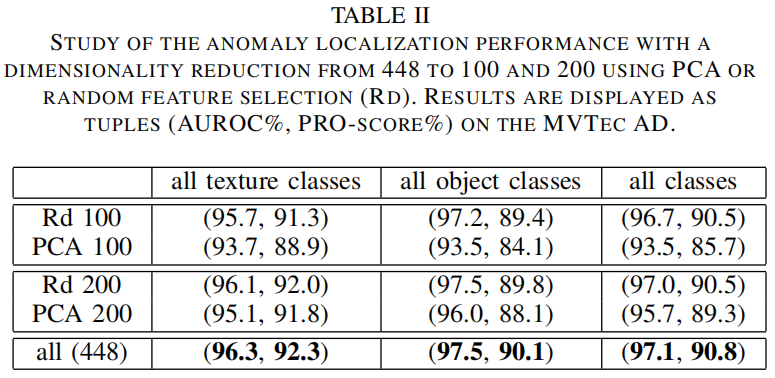
作者对比了PCA和随机挑选两种降维方法，通过上表可以看出，无论降到100维还是200维，随机挑选的效果都比PCA好，这可能是因为PCA挑选的是那些方差最大的维度，但这些维度可能不是最有助于区分正常和异常类的维度。另外随机挑选的方法从448维将到200维再降到100维，精度损失都不大，但却大大降低了模型复杂度。 

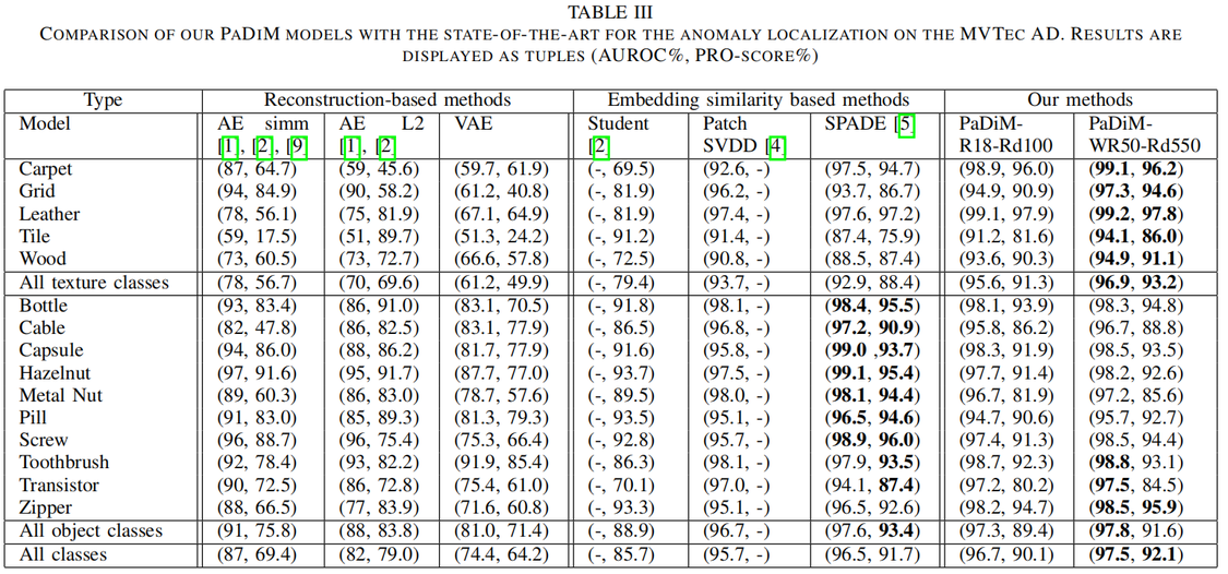
Comparison with the state-of-the-art