
学习参考来自
- Saliency Maps的原理与简单实现(使用Pytorch实现)
- https://github.com/wmn7/ML_Practice/tree/master/2019_07_08/Saliency%20Maps
Saliency Maps 原理
《Deep Inside Convolutional Networks: Visualising Image Classification Models and Saliency Maps》(arXiv-2013)
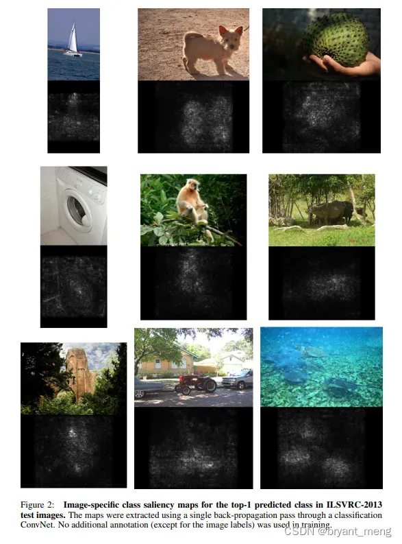
A saliency map tells us the degree to which each pixel in the image affects the classification score for that image.
To compute it, we compute the gradient of the unnormalized score corresponding to the correct class (which is a scalar)
with respect to the pixels of the image. If the image has shape (3, H, W) then this gradient will also have shape (3, H, W);
for each pixel in the image, this gradient tells us the amount by which the classification score will change if the pixel
changes by a small amount. To compute the saliency map, we take the absolute value of this gradient, then take the maximum value over the 3 input channels; the final saliency map thus has shape (H, W) and all entries are non-negative.
Saliency Maps相当于是计算图像的每一个pixel是如何影响一个分类器的, 或者说分类器对图像中每一个pixel哪些认为是重要的.
会计算图像每一个像素点的梯度。如果图像的形状是(3, H, W),这个梯度的形状也是(3, H, W);对于图像中的每个像素点,
这个梯度告诉我们当像素点发生轻微改变时,正确分类分数变化的幅度。
计算 saliency map 的时候,需要计算出梯度的绝对值,然后再取三个颜色通道的最大值;
因此最后的 saliency map的形状是(H, W)为一个通道的灰度图。
直接来代码,先载入些数据,用的是 cs231n 作业里面的 imagenet_val_25.npz,含有 imagenet 数据中验证集的 25 张图片
import torch
import torchvision
import torchvision.transforms as T
import matplotlib.pyplot as plt
import numpy as np
import os
from PIL import Image

SQUEEZENET_MEAN = np.array([0.485, 0.456, 0.406], dtype=np.float32)
SQUEEZENET_STD = np.array([0.229, 0.224, 0.225], dtype=np.float32)

def load_imagenet_val(num=None):
    """Load a handful of validation images from ImageNet.
    Inputs:
    - num: Number of images to load (max of 25)
    Returns:
    - X: numpy array with shape [num, 224, 224, 3]
    - y: numpy array of integer image labels, shape [num]
    - class_names: dict mapping integer label to class name
    """
    imagenet_fn = 'imagenet_val_25.npz'
    if not os.path.isfile(imagenet_fn):
      print('file %s not found' % imagenet_fn)
      print('Run the following:')
      print('cd cs231n/datasets')
      print('bash get_imagenet_val.sh')
      assert False, 'Need to download imagenet_val_25.npz'
    f = np.load(imagenet_fn, allow_pickle=True)
    X = f['X']  # (25, 224, 224, 3)
    y = f['y']  # (25, )
    class_names = f['label_map'].item()  # 999
    if num is not None:
        X = X[:num]
        y = y[:num]
    return X, y, class_names
图像的前处理,resize,变成向量,减均值除以方差
# 辅助函数
def preprocess(img, size=224):
    transform = T.Compose([
        T.Resize(size),
        T.ToTensor(),
        T.Normalize(mean=SQUEEZENET_MEAN.tolist(),
                    std=SQUEEZENET_STD.tolist()),
        T.Lambda(lambda x: x[None]),
    ])
    return transform(img)
数据集和实验的模型
链接:https://pan.baidu.com/s/1vb2Y0IiHdH_Fb9wibTta4Q?pwd=zuvw
提取码:zuvw
核心代码,计算 saliency maps
def compute_saliency_maps(X, y, model):
    """
    X表示图片, y表示分类结果, model表示使用的分类模型

    Input :
    - X : Input images : Tensor of shape (N, 3, H, W)
    - y : Label for X : LongTensor of shape (N,)
    - model : A pretrained CNN that will be used to computer the saliency map

    Return :
    - saliency : A Tensor of shape (N, H, W) giving the saliency maps for the input images
    """
    # 确保model是test模式
    model.eval()

    # 确保X是需要gradient
    X.requires_grad_() # 仅开启了输入图片的梯度

    saliency = None

    logits = model.forward(X)  # torch.Size([5, 1000]), 前向获取 logits
    logits = logits.gather(1, y.view(-1, 1)).squeeze()  # torch.Size([5]) 得到正确分类 logits (5张图片标签相应类别的 logits)
    logits.backward(torch.FloatTensor([1., 1., 1., 1., 1.]))  # 只计算正确分类部分的loss(正确类别梯度为 1 回传)

    saliency = abs(X.grad.data)  # 返回X的梯度绝对值大小, torch.Size([5, 3, 224, 224])
    saliency, _ = torch.max(saliency, dim=1)  # torch.Size([5, 224, 224]),取 rgb 3通道的最大值

    return saliency.squeeze()
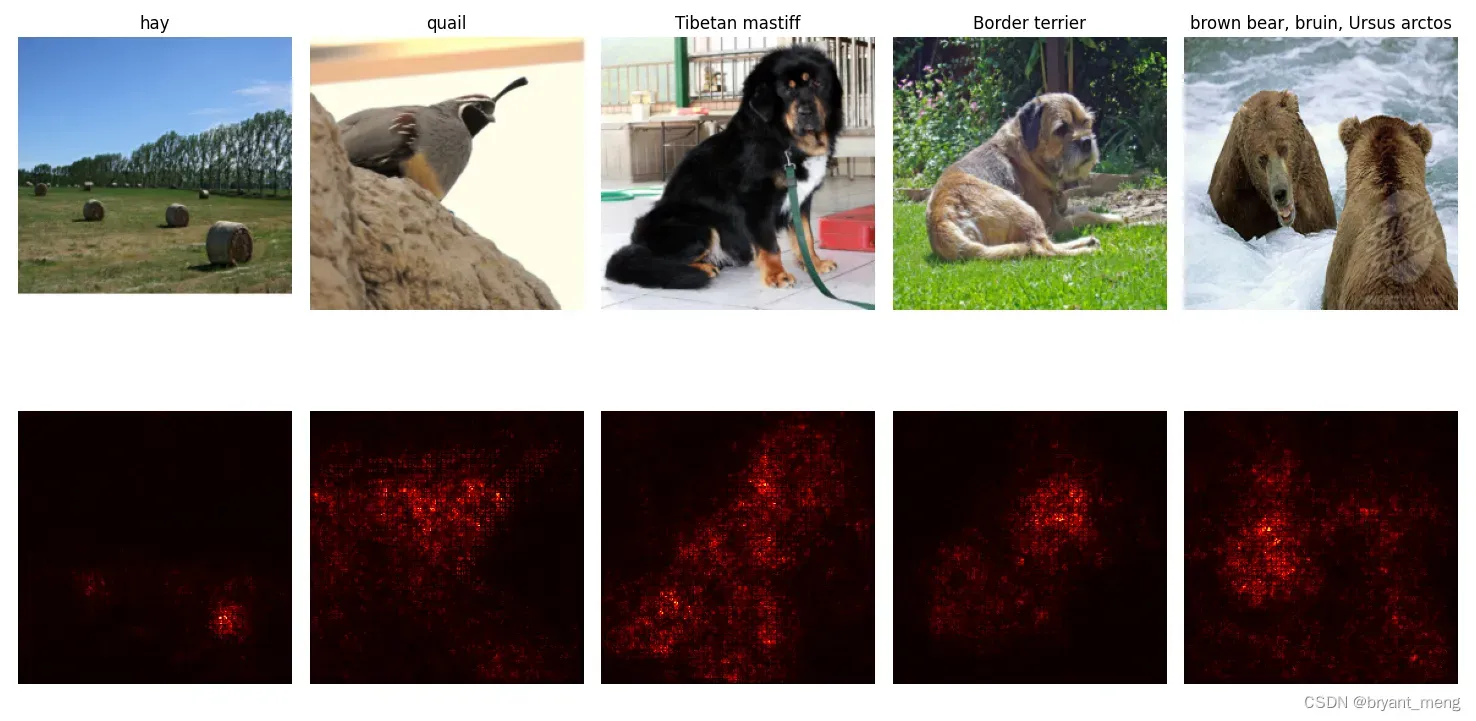
显示 saliency maps
def show_saliency_maps(X, y):
    # Convert X and y from numpy arrays to Torch Tensors
    X_tensor = torch.cat([preprocess(Image.fromarray(x)) for x in X], dim=0) # torch.Size([5, 3, 224, 224])
    y_tensor = torch.LongTensor(y)

    # Compute saliency maps for images in X
    saliency = compute_saliency_maps(X_tensor, y_tensor, model)

    # Convert the saliency map from Torch Tensor to numpy array and show images
    # and saliency maps together.
    saliency = saliency.numpy()
    N = X.shape[0]  # 5
    for i in range(N):
        plt.subplot(2, N, i + 1)
        plt.imshow(X[i])
        plt.axis('off')
        plt.title(class_names[y[i]])
        plt.subplot(2, N, N + i + 1)
        plt.imshow(saliency[i], cmap=plt.cm.hot)
        plt.axis('off')
        plt.gcf().set_size_inches(12, 5)
    plt.show()
下面开始调用,首先载入模型,使其梯度冻结,仅打开输入图片的梯度,这样反向传播的时候会更新图片,得到我们想要的 saliency maps
# Download and load the pretrained SqueezeNet model.
model = torchvision.models.squeezenet1_1(pretrained=True)

# We don't want to train the model, so tell PyTorch not to compute gradients
# with respect to model parameters.
for param in model.parameters():
    param.requires_grad = False
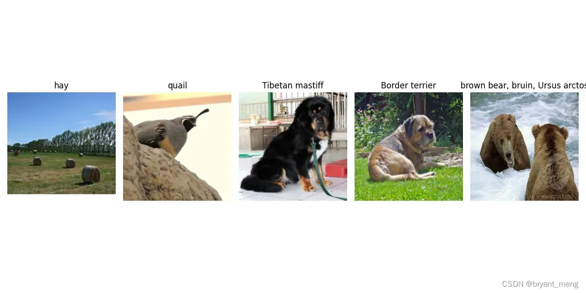
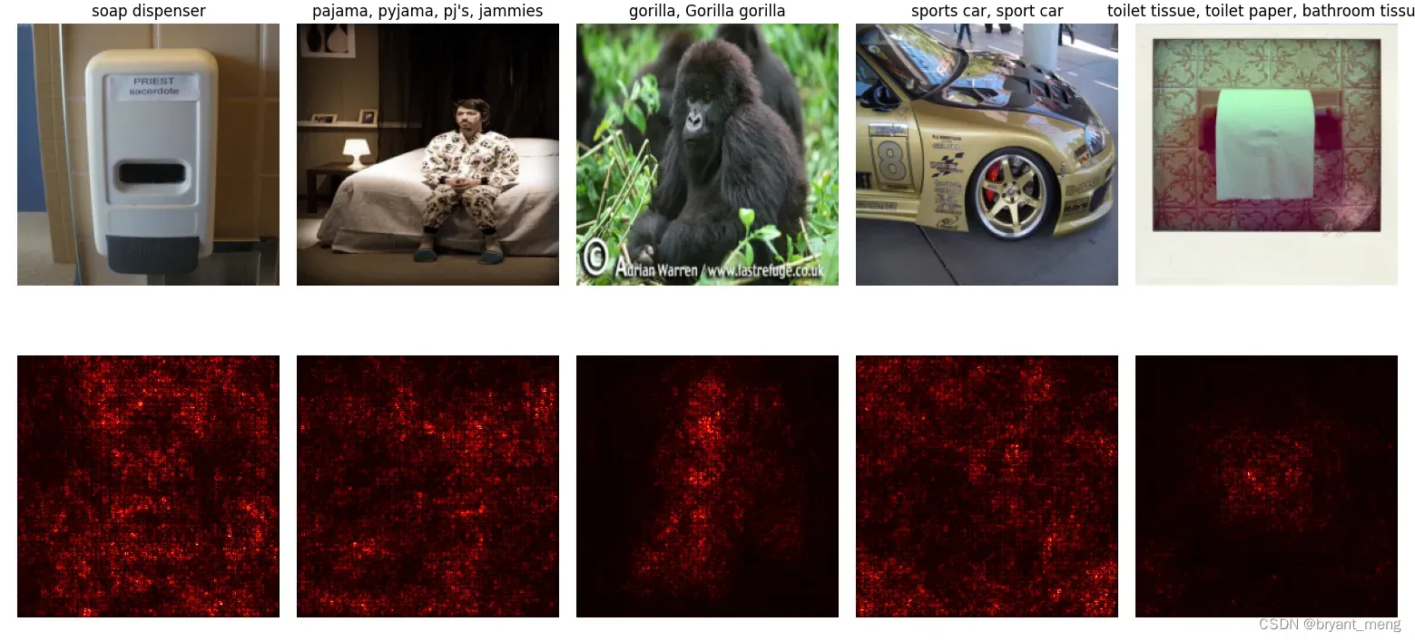
加载一些图片看看,25 张中抽出来 5 张
X, y, class_names = load_imagenet_val(num=5)  # X: (5, 224, 224, 3) | y: (5,) | class_names: 999

"show images"

plt.figure(figsize=(12, 6))
for i in range(5):
    plt.subplot(1, 5, i + 1)
    plt.imshow(X[i])
    plt.title(class_names[y[i]])
    plt.axis('off')
plt.gcf().tight_layout()
plt.show()
显示图片
把五张图片的 saliency maps 画出来
show_saliency_maps(X, y)
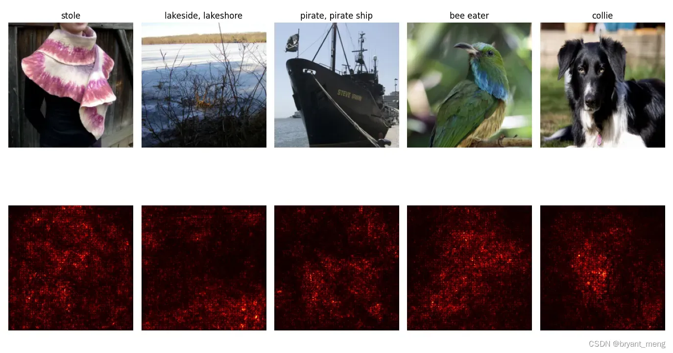
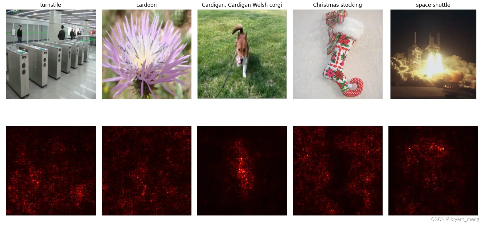
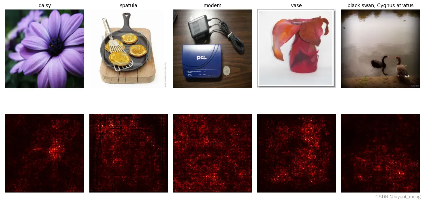
我把 25 张都画出来了
核心代码中涉及到了 gather 函数,下面来个简单的例子就明白了
# Example of using gather to select one entry from each row in PyTorch
# 用来返回matrix指定行某个位置的值
import torch

def gather_example():
    N, C = 4, 5
    s = torch.randn(N, C) # 随机生成 4 行 5 列的 tensor
    y = torch.LongTensor([1, 2, 1, 3])
    print(s)
    print(y)
    print(torch.LongTensor(y).view(-1, 1))
    print(s.gather(1, y.view(-1, 1)).squeeze()) # 抽取每行相应的列数位置上的数值


gather_example()

"""
tensor([[ 0.8119,  0.2664, -1.4168, -0.1490, -0.0675],
        [ 0.5335,  0.6304, -0.7200, -0.0974, -0.9934],
        [-0.8305,  0.5189,  0.7359,  1.5875,  0.0505],
        [ 0.4335, -1.1389, -0.7771,  0.5779,  0.3515]])
tensor([1, 2, 1, 3])
tensor([[1],
        [2],
        [1],
        [3]])
tensor([ 0.2664, -0.7200,  0.5189,  0.5779])
"""
文章出处登录后可见!