1. Introduction
Midjourney,Stable Diffusion,DALL-E等产品能够仅通过Prompt就能够生成图像。本课程将介绍这些应用背后算法的原理。
课程地址:https://learn.deeplearning.ai/diffusion-models/
2. Intuition
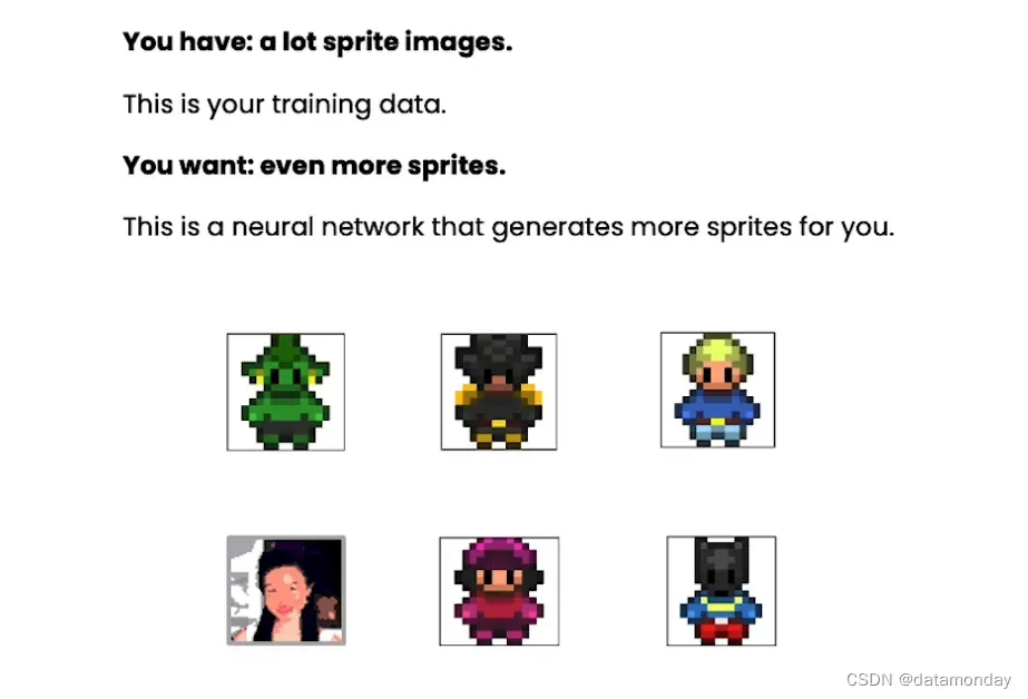
本小节将介绍扩散模型的基础知识,探讨扩散模型的目标,如何利用各种游戏角色图片训练数据来增强模型的能力。
假设下面是你的数据集,你想要更多的在这些数据集中没有的角色图片,如何做到?可以使用扩散模型生成这样的角色图片。
扩散模型应该是这样的一个神经网络:它能够学习到游戏角色的一般概念,例如游戏角色是什么,游戏角色的身体轮廓等等,甚至是更细微的细节,例如游戏角色的头发颜色或者腰带扣。
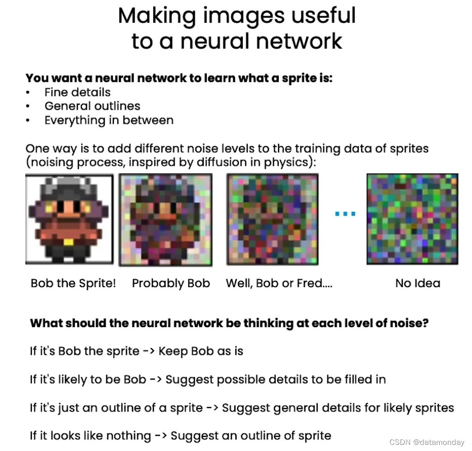
有一种方法可以做到这一点,就是在训练数据上添加不同程度的噪声,这被称为噪声过程(noising process),这是时受到物理学的启发而取的名字。你可以想象一滴墨水滴入一杯水中,随着时间的推移,它会在水中扩散,直至消失。当你逐渐给图像添加更多的噪声时,图片的轮廓从清晰变模糊,直到完全无法辨别。这个逐渐添加不同程度噪声的过程很像墨水在水中逐渐消失的过程。
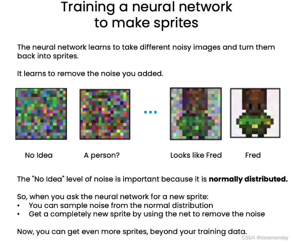
训练模型的目标是:模型会移除你添加的噪声,将添加了不同噪声的图像变换为游戏角色。
3. Sampling
采样是神经网络训练完成之后,在推理时做的事。
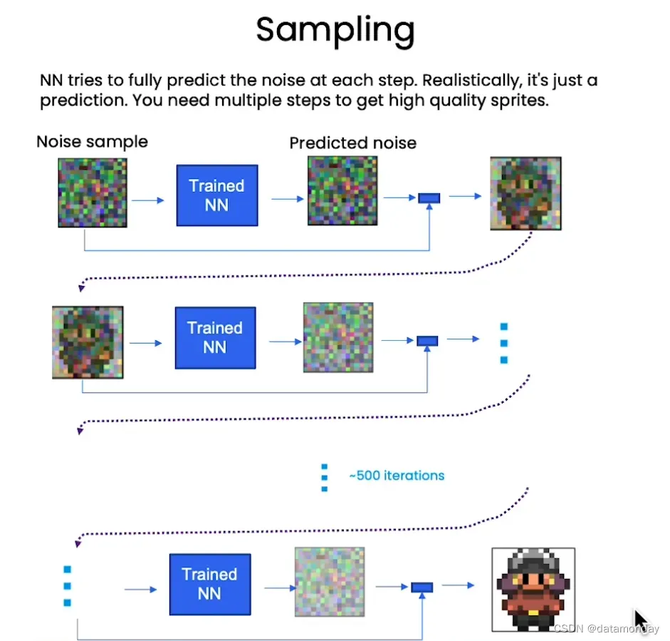
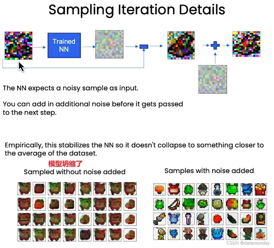
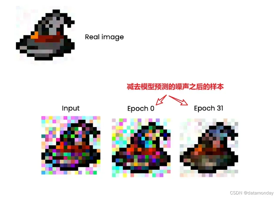
假设有一个已经添加了噪声的样本,将其输入到已经训练好的神经网络中,这个神经网络已经理解了游戏角色图片。之后,让神经网络预测噪声,然后,从噪声样本中减去预测的噪声,得到的结果就更接近游戏角色图片。
现实情况是,这只是对噪声的预测,并没有完全消除所有的噪声,需要迭代很多次在能够得到接近原始图片的高质量的样本。
下面是采样算法的实现:
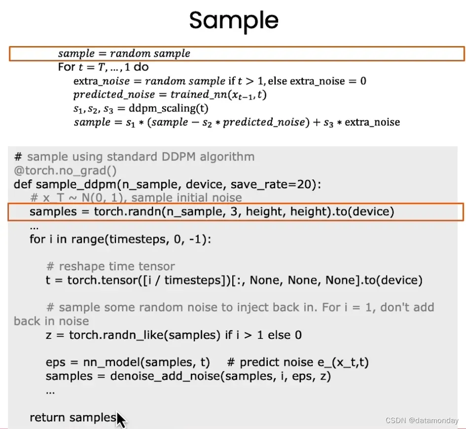
首先可以采样一个随机噪声样本,这就是一开始的原始噪声,然后逆序从最后一次迭代的完全噪声的状态遍历到第一次迭代。就像时光倒流,也可以想象是墨水的例子,一开始完全扩散的,然后一直倒退回到刚刚滴入水中的状态。
之后,采样一些特殊的噪声。
之后,将原始的噪声再次输入到神经网络,然后得到一些预测的噪声。这个预测的噪声就是训练过的神经网络想从原始噪声中减去的噪声,从而得到更像原始的游戏角色的图片。
最后,通过降噪扩散概率模型(Denoising Diffusion Probabilistic Models,DDPM)得到从原始噪声中减去预测的噪声,再加上一些额外的噪声。
from typing import Dict, Tuple
from tqdm import tqdm
import torch
import torch.nn as nn
import torch.nn.functional as F
from torch.utils.data import DataLoader
from torchvision import models, transforms
from torchvision.utils import save_image, make_grid
import matplotlib.pyplot as plt
from matplotlib.animation import FuncAnimation, PillowWriter
import numpy as np
from IPython.display import HTML
from diffusion_utilities import *

class ContextUnet(nn.Module):
    def __init__(self, in_channels, n_feat=256, n_cfeat=10, height=28):  # cfeat - context features
        super(ContextUnet, self).__init__()

        # number of input channels, number of intermediate feature maps and number of classes
        self.in_channels = in_channels
        self.n_feat = n_feat
        self.n_cfeat = n_cfeat
        self.h = height  #assume h == w. must be divisible by 4, so 28,24,20,16...

        # Initialize the initial convolutional layer
        self.init_conv = ResidualConvBlock(in_channels, n_feat, is_res=True)

        # Initialize the down-sampling path of the U-Net with two levels
        self.down1 = UnetDown(n_feat, n_feat)        # down1 #[10, 256, 8, 8]
        self.down2 = UnetDown(n_feat, 2 * n_feat)    # down2 #[10, 256, 4,  4]

         # original: self.to_vec = nn.Sequential(nn.AvgPool2d(7), nn.GELU())
        self.to_vec = nn.Sequential(nn.AvgPool2d((4)), nn.GELU())

        # Embed the timestep and context labels with a one-layer fully connected neural network
        self.timeembed1 = EmbedFC(1, 2*n_feat)
        self.timeembed2 = EmbedFC(1, 1*n_feat)
        self.contextembed1 = EmbedFC(n_cfeat, 2*n_feat)
        self.contextembed2 = EmbedFC(n_cfeat, 1*n_feat)

        # Initialize the up-sampling path of the U-Net with three levels
        self.up0 = nn.Sequential(
            nn.ConvTranspose2d(2 * n_feat, 2 * n_feat, self.h//4, self.h//4), # up-sample
            nn.GroupNorm(8, 2 * n_feat), # normalize
            nn.ReLU(),
        )
        self.up1 = UnetUp(4 * n_feat, n_feat)
        self.up2 = UnetUp(2 * n_feat, n_feat)

        # Initialize the final convolutional layers to map to the same number of channels as the input image
        self.out = nn.Sequential(
            nn.Conv2d(2 * n_feat, n_feat, 3, 1, 1), # reduce number of feature maps   #in_channels, out_channels, kernel_size, stride=1, padding=0
            nn.GroupNorm(8, n_feat), # normalize
            nn.ReLU(),
            nn.Conv2d(n_feat, self.in_channels, 3, 1, 1), # map to same number of channels as input
        )

    def forward(self, x, t, c=None):
        """
        x : (batch, n_feat, h, w) : input image
        t : (batch, n_cfeat)      : time step
        c : (batch, n_classes)    : context label
        """
        # x is the input image, c is the context label, t is the timestep, context_mask says which samples to block the context on

        # pass the input image through the initial convolutional layer
        x = self.init_conv(x)
        # pass the result through the down-sampling path
        down1 = self.down1(x)       #[10, 256, 8, 8]
        down2 = self.down2(down1)   #[10, 256, 4, 4]

        # convert the feature maps to a vector and apply an activation
        hiddenvec = self.to_vec(down2)

        # mask out context if context_mask == 1
        if c is None:
            c = torch.zeros(x.shape[0], self.n_cfeat).to(x)

        # embed context and timestep
        cemb1 = self.contextembed1(c).view(-1, self.n_feat * 2, 1, 1)     # (batch, 2*n_feat, 1,1)
        temb1 = self.timeembed1(t).view(-1, self.n_feat * 2, 1, 1)
        cemb2 = self.contextembed2(c).view(-1, self.n_feat, 1, 1)
        temb2 = self.timeembed2(t).view(-1, self.n_feat, 1, 1)
        #print(f"uunet forward: cemb1 {cemb1.shape}. temb1 {temb1.shape}, cemb2 {cemb2.shape}. temb2 {temb2.shape}")


        up1 = self.up0(hiddenvec)
        up2 = self.up1(cemb1*up1 + temb1, down2)  # add and multiply embeddings
        up3 = self.up2(cemb2*up2 + temb2, down1)
        out = self.out(torch.cat((up3, x), 1))
        return out
# hyperparameters

# diffusion hyperparameters
timesteps = 500
beta1 = 1e-4
beta2 = 0.02

# network hyperparameters
device = torch.device("cuda:0" if torch.cuda.is_available() else torch.device('cpu'))
n_feat = 64 # 64 hidden dimension feature
n_cfeat = 5 # context vector is of size 5
height = 16 # 16x16 image
save_dir = './weights/'

# construct DDPM noise schedule
b_t = (beta2 - beta1) * torch.linspace(0, 1, timesteps + 1, device=device) + beta1
a_t = 1 - b_t
ab_t = torch.cumsum(a_t.log(), dim=0).exp()
ab_t[0] = 1

# construct model
nn_model = ContextUnet(in_channels=3, n_feat=n_feat, n_cfeat=n_cfeat, height=height).to(device)
超参数介绍:
- beta1:DDPM算法的超参数;
- beta2:DDPM算法的超参数;
- height:图片的长度和高度;
- noise schedule(噪声调度):确定在某个时间步长应用于图像的噪声级别;
- S1,S2,S3:缩放因子的值
# helper function; removes the predicted noise (but adds some noise back in to avoid collapse)
def denoise_add_noise(x, t, pred_noise, z=None):
    if z is None:
        z = torch.randn_like(x)
    noise = b_t.sqrt()[t] * z
    mean = (x - pred_noise * ((1 - a_t[t]) / (1 - ab_t[t]).sqrt())) / a_t[t].sqrt()
    return mean + noise

# load in model weights and set to eval mode
nn_model.load_state_dict(torch.load(f"{save_dir}/model_trained.pth", map_location=device))
nn_model.eval()
print("Loaded in Model")


# sample using standard algorithm
@torch.no_grad()
def sample_ddpm(n_sample, save_rate=20):
    # x_T ~ N(0, 1), sample initial noise
    samples = torch.randn(n_sample, 3, height, height).to(device)

    # array to keep track of generated steps for plotting
    intermediate = []
    for i in range(timesteps, 0, -1):
        print(f'sampling timestep {i:3d}', end='\r')

        # reshape time tensor
        t = torch.tensor([i / timesteps])[:, None, None, None].to(device)

        # sample some random noise to inject back in. For i = 1, don't add back in noise
        # 这里设置为0,会导致模型坍缩
        z = torch.randn_like(samples) if i > 1 else 0

        eps = nn_model(samples, t)    # predict noise e_(x_t,t)
        samples = denoise_add_noise(samples, i, eps, z)
        if i % save_rate ==0 or i==timesteps or i<8:
            intermediate.append(samples.detach().cpu().numpy())

    intermediate = np.stack(intermediate)
    return samples, intermediate
# visualize samples
plt.clf()
samples, intermediate_ddpm = sample_ddpm(32)
animation_ddpm = plot_sample(intermediate_ddpm,32,4,save_dir, "ani_run", None, save=False)
HTML(animation_ddpm.to_jshtml())

需要注意的是,神经网络的输入需要的是符合正态分布的噪声样本。在迭代过程中,噪声样本减去模型预测的噪声之后得到的样本已经不符合正态分布了,容易导致模型坍缩。所以每次迭代之后需要根据所处的时间步长添加额外的采样噪声,以让其符合正态分布。从经验上看,这可以保证训练的稳定性,以避免模型模型坍缩,导致模型的预测结果接近于数据集的平均值。
4. Neural Network
用于扩散模型的神经网络架构是U-Net。它将原始图像作为输入,输出与原始图像大小相同的预测噪声。输入与输出尺寸相同,这是其一大优点。
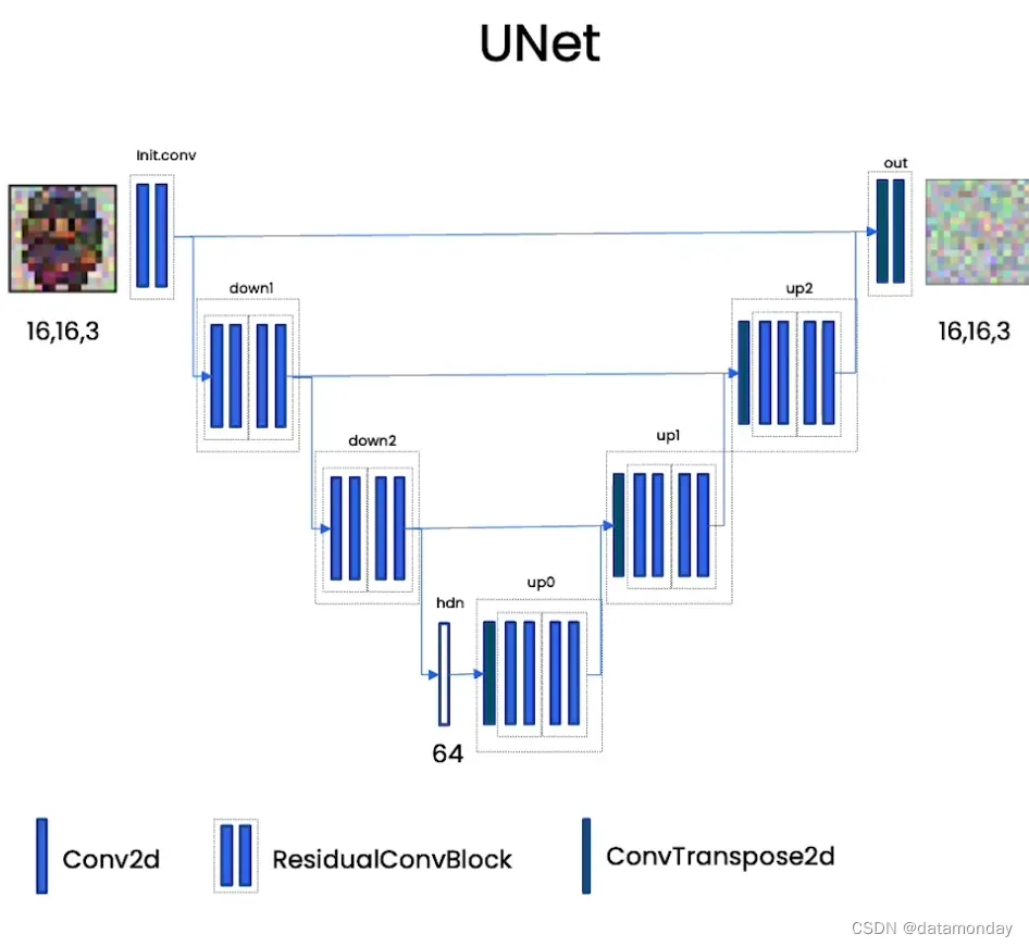
U-Net首先将这个输入的信息进行嵌入(Embedding),通过多层卷积将其降采样到一个压缩了所有信息的嵌入(Embedding)中。然后用相同数量的上采样块将输出返回到任务中,在这个例子中,它的任务就是预测应用到这个图片上的噪声。
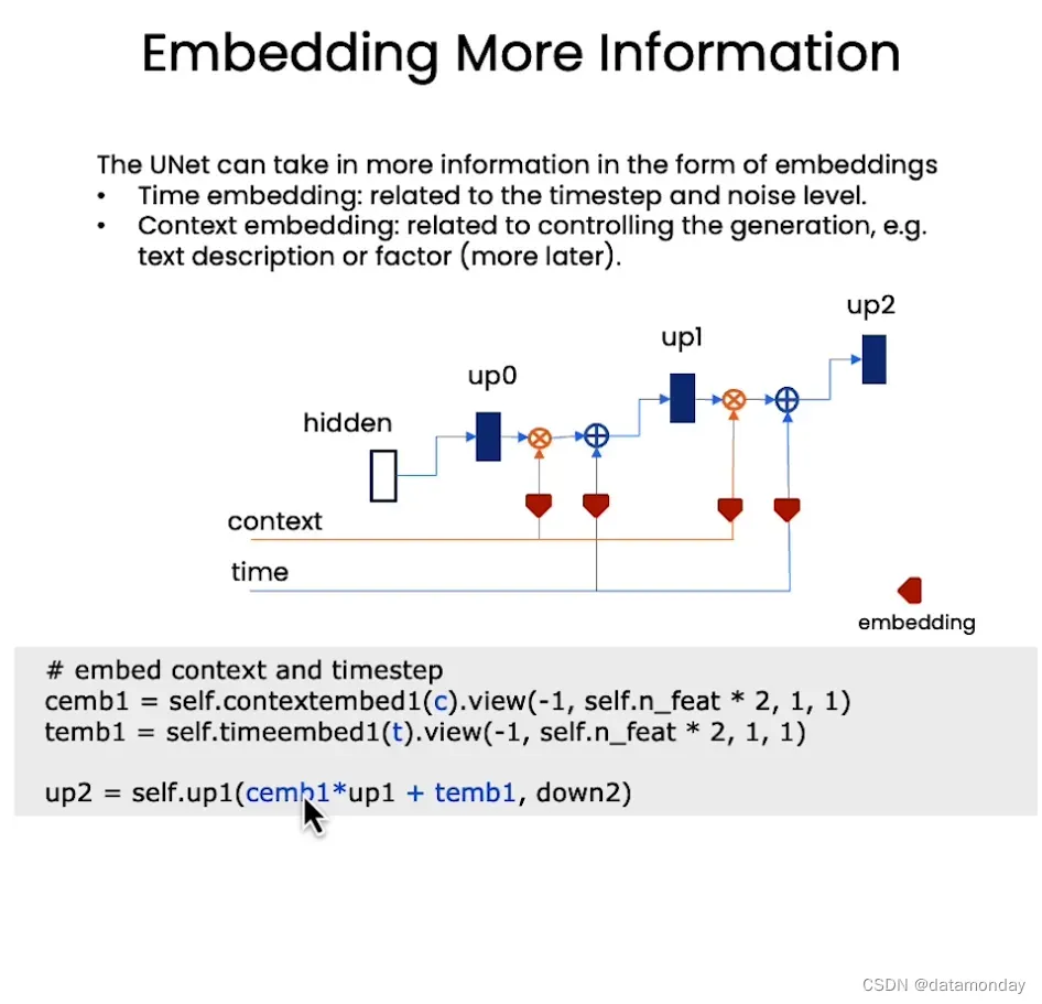
U-Net的另一个优点是可以接受额外的信息,所以它压缩了图像以了解发生了什么,但也可以接收更多的信息。那么我们需要哪些额外的信息呢?
对于这些模型来说,一个非常重要的信息就是时间嵌入(Time Embedding),这是一种告诉模型时间步长的嵌入,因此我们需要某种级别的噪声。对于这个时间嵌入,需要将其嵌入到一个向量中,然后将其添加到这些上采样块中。
另一个非常重要的信息是上下文嵌入(Context Embedding),它的根本作用是控制模型生成的内容。例如,一个文本描述,你想让它生成的是Bob,或者某种因子,或者某种颜色。具体到代码实现如下:
5. Training
训练神经网络(NN)的目标是让网络预测噪声,真正的任务是让它学习图像上的噪声分布(也包括需要学习什么是游戏角色图片的特征)。
训练策略是:从训练数据中去一张游戏角色图片,然后添加随机噪声,然后让NN预测这个噪声。之后,将预测的噪声与实际的噪声进行比较,计算损失函数。通过BP算法不断迭代,让NN学会更好的预测噪声。
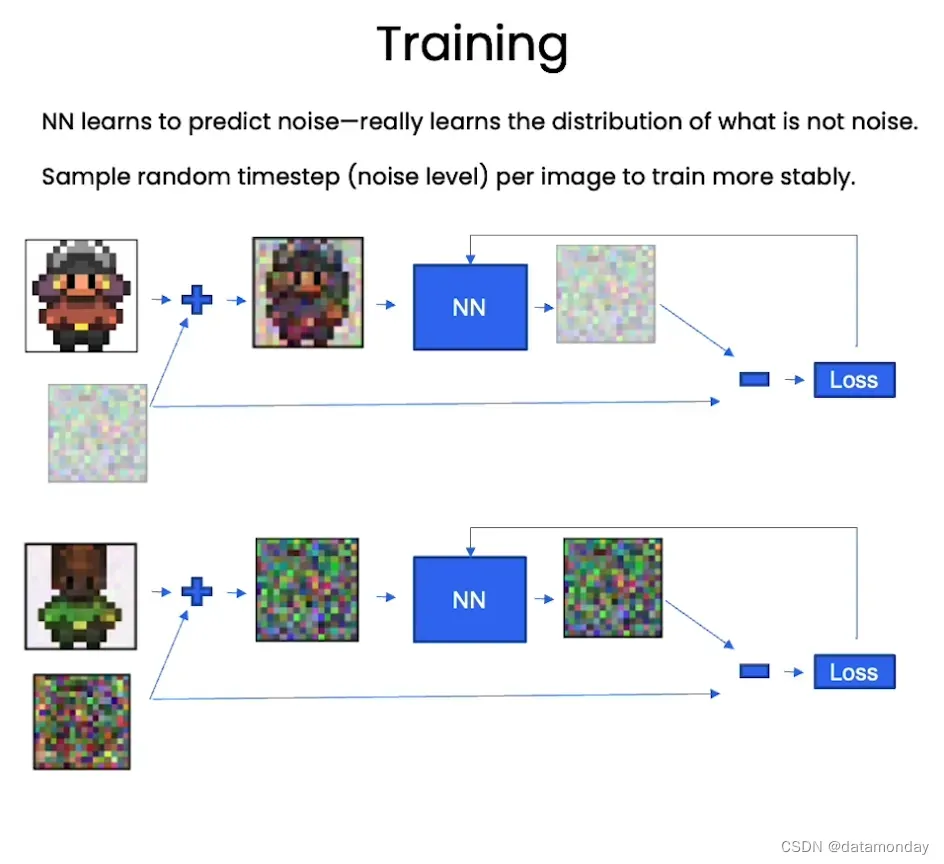
那么如何确定这里的噪声是什么?
可以通过时间和采样,给它不同的噪声级别。但在实际的训练过程中,我们不希望NN一直观察同一个游戏角色图片,因为如果在一个周期内观察到不同的游戏角色图片,NN会更稳定,更均匀。所以,我们实际上是随机采样一个可能的时间步长,然后获取相应的噪声级别,添加到图像中,再让NN做预测。
之后,选择下一张游戏角色图片,执行同样的过程。这样就得到了一个稳定的训练过程。
# load dataset and construct optimizer
dataset = CustomDataset("./sprites_1788_16x16.npy", "./sprite_labels_nc_1788_16x16.npy", transform, null_context=False)
dataloader = DataLoader(dataset, batch_size=batch_size, shuffle=True, num_workers=1)
optim = torch.optim.Adam(nn_model.parameters(), lr=lrate)
# helper function: perturbs an image to a specified noise level
def perturb_input(x, t, noise):
    return ab_t.sqrt()[t, None, None, None] * x + (1 - ab_t[t, None, None, None]) * noise
# training without context code

# set into train mode
nn_model.train()

for ep in range(n_epoch):
    print(f'epoch {ep}')

    # linearly decay learning rate
    optim.param_groups[0]['lr'] = lrate*(1-ep/n_epoch)

    pbar = tqdm(dataloader, mininterval=2 )
    for x, _ in pbar:   # x: images
        optim.zero_grad()
        x = x.to(device)

        # perturb data
        noise = torch.randn_like(x)
        t = torch.randint(1, timesteps + 1, (x.shape[0],)).to(device)
        x_pert = perturb_input(x, t, noise)

        # use network to recover noise
        pred_noise = nn_model(x_pert, t / timesteps)

        # loss is mean squared error between the predicted and true noise
        loss = F.mse_loss(pred_noise, noise)
        loss.backward()

        optim.step()

    # save model periodically
    if ep%4==0 or ep == int(n_epoch-1):
        if not os.path.exists(save_dir):
            os.mkdir(save_dir)
        torch.save(nn_model.state_dict(), save_dir + f"model_{ep}.pth")
        print('saved model at ' + save_dir + f"model_{ep}.pth")
# load in model weights and set to eval mode
nn_model.load_state_dict(torch.load(f"{save_dir}/model_0.pth", map_location=device))
nn_model.eval()
print("Loaded in Model")
# visualize samples
plt.clf()
samples, intermediate_ddpm = sample_ddpm(32)
animation_ddpm = plot_sample(intermediate_ddpm,32,4,save_dir, "ani_run", None, save=False)
HTML(animation_ddpm.to_jshtml())
6. Controlling
本小节介绍如何控制模型生成的内容。
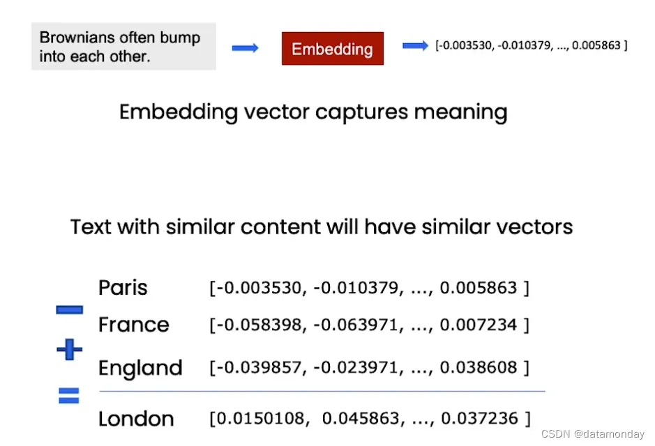
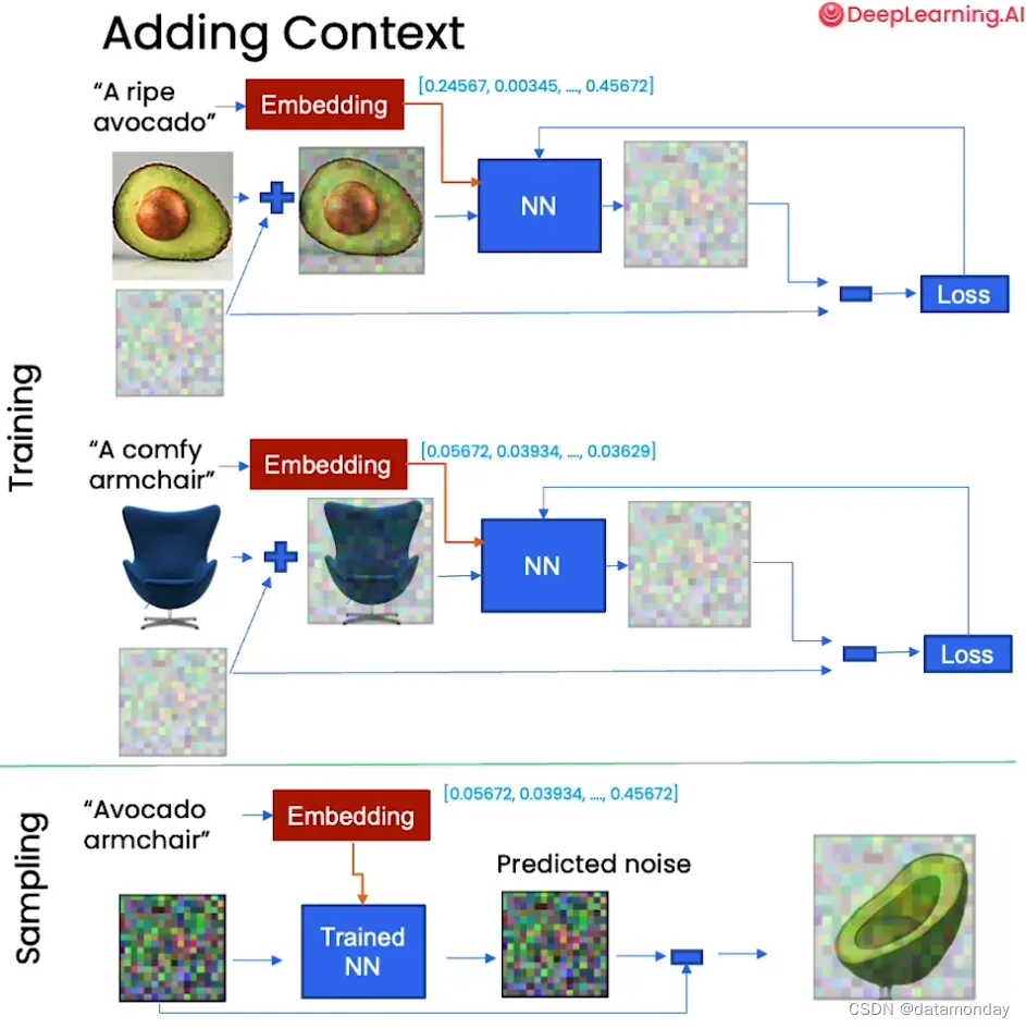
在想控制这些模型时,需要使用嵌入(Embeddings)。嵌入的特殊之处在它可以捕获文本的语义,内容相似的文本具有相似的向量。并且可以对向量进行算术运算,例如,将巴黎的嵌入减去法国的嵌入,加上英国的嵌入,等于伦敦的嵌入。
那么在训练过程中,这些嵌入是如何成为模型上下文的呢?将图片的标题文本转换成Embedding,随原始的图片一起输入到NN中,这也就构成了上下文的一部分。
扩散模型的神奇之处在于,在进行采样时,可以生成数据集中没有的东西,例如下面的例子中,输入“牛油果扶手椅”的文本Embedding,最终模型生成了一个牛油果做成的扶手椅。
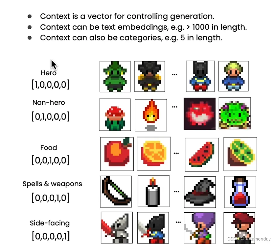
从更广泛的意义上来看,上下文可以是一个控制NN生成的向量。除了文本Embedding当做上下文以外,也可以将one-hot编码后的图片类别当做上下文。
from typing import Dict, Tuple
from tqdm import tqdm
import torch
import torch.nn as nn
import torch.nn.functional as F
from torch.utils.data import DataLoader
from torchvision import models, transforms
from torchvision.utils import save_image, make_grid
import matplotlib.pyplot as plt
from matplotlib.animation import FuncAnimation, PillowWriter
import numpy as np
from IPython.display import HTML
from diffusion_utilities import *


class ContextUnet(nn.Module):
    def __init__(self, in_channels, n_feat=256, n_cfeat=10, height=28):  # cfeat - context features
        super(ContextUnet, self).__init__()

        # number of input channels, number of intermediate feature maps and number of classes
        self.in_channels = in_channels
        self.n_feat = n_feat
        self.n_cfeat = n_cfeat
        self.h = height  #assume h == w. must be divisible by 4, so 28,24,20,16...

        # Initialize the initial convolutional layer
        self.init_conv = ResidualConvBlock(in_channels, n_feat, is_res=True)

        # Initialize the down-sampling path of the U-Net with two levels
        self.down1 = UnetDown(n_feat, n_feat)        # down1 #[10, 256, 8, 8]
        self.down2 = UnetDown(n_feat, 2 * n_feat)    # down2 #[10, 256, 4,  4]

         # original: self.to_vec = nn.Sequential(nn.AvgPool2d(7), nn.GELU())
        self.to_vec = nn.Sequential(nn.AvgPool2d((4)), nn.GELU())

        # Embed the timestep and context labels with a one-layer fully connected neural network
        self.timeembed1 = EmbedFC(1, 2*n_feat)
        self.timeembed2 = EmbedFC(1, 1*n_feat)
        self.contextembed1 = EmbedFC(n_cfeat, 2*n_feat)
        self.contextembed2 = EmbedFC(n_cfeat, 1*n_feat)

        # Initialize the up-sampling path of the U-Net with three levels
        self.up0 = nn.Sequential(
            nn.ConvTranspose2d(2 * n_feat, 2 * n_feat, self.h//4, self.h//4), # up-sample
            nn.GroupNorm(8, 2 * n_feat), # normalize
            nn.ReLU(),
        )
        self.up1 = UnetUp(4 * n_feat, n_feat)
        self.up2 = UnetUp(2 * n_feat, n_feat)

        # Initialize the final convolutional layers to map to the same number of channels as the input image
        self.out = nn.Sequential(
            nn.Conv2d(2 * n_feat, n_feat, 3, 1, 1), # reduce number of feature maps   #in_channels, out_channels, kernel_size, stride=1, padding=0
            nn.GroupNorm(8, n_feat), # normalize
            nn.ReLU(),
            nn.Conv2d(n_feat, self.in_channels, 3, 1, 1), # map to same number of channels as input
        )

    def forward(self, x, t, c=None):
        """
        x : (batch, n_feat, h, w) : input image
        t : (batch, n_cfeat)      : time step
        c : (batch, n_classes)    : context label
        """
        # x is the input image, c is the context label, t is the timestep, context_mask says which samples to block the context on

        # pass the input image through the initial convolutional layer
        x = self.init_conv(x)
        # pass the result through the down-sampling path
        down1 = self.down1(x)       #[10, 256, 8, 8]
        down2 = self.down2(down1)   #[10, 256, 4, 4]

        # convert the feature maps to a vector and apply an activation
        hiddenvec = self.to_vec(down2)

        # mask out context if context_mask == 1
        if c is None:
            c = torch.zeros(x.shape[0], self.n_cfeat).to(x)

        # embed context and timestep
        cemb1 = self.contextembed1(c).view(-1, self.n_feat * 2, 1, 1)     # (batch, 2*n_feat, 1,1)
        temb1 = self.timeembed1(t).view(-1, self.n_feat * 2, 1, 1)
        cemb2 = self.contextembed2(c).view(-1, self.n_feat, 1, 1)
        temb2 = self.timeembed2(t).view(-1, self.n_feat, 1, 1)
        #print(f"uunet forward: cemb1 {cemb1.shape}. temb1 {temb1.shape}, cemb2 {cemb2.shape}. temb2 {temb2.shape}")


        up1 = self.up0(hiddenvec)
        up2 = self.up1(cemb1*up1 + temb1, down2)  # add and multiply embeddings
        up3 = self.up2(cemb2*up2 + temb2, down1)
        out = self.out(torch.cat((up3, x), 1))
        return out
# hyperparameters

# diffusion hyperparameters
timesteps = 500
beta1 = 1e-4
beta2 = 0.02

# network hyperparameters
device = torch.device("cuda:0" if torch.cuda.is_available() else torch.device('cpu'))
n_feat = 64 # 64 hidden dimension feature
n_cfeat = 5 # context vector is of size 5
height = 16 # 16x16 image
save_dir = './weights/'

# training hyperparameters
batch_size = 100
n_epoch = 32
lrate=1e-3

# construct DDPM noise schedule
b_t = (beta2 - beta1) * torch.linspace(0, 1, timesteps + 1, device=device) + beta1
a_t = 1 - b_t
ab_t = torch.cumsum(a_t.log(), dim=0).exp()
ab_t[0] = 1

# construct model
nn_model = ContextUnet(in_channels=3, n_feat=n_feat, n_cfeat=n_cfeat, height=height).to(device)
设置上下文
# reset neural network
nn_model = ContextUnet(in_channels=3, n_feat=n_feat, n_cfeat=n_cfeat, height=height).to(device)

# re setup optimizer
optim = torch.optim.Adam(nn_model.parameters(), lr=lrate)
训练
# training with context code
# set into train mode
nn_model.train()

for ep in range(n_epoch):
    print(f'epoch {ep}')

    # linearly decay learning rate
    optim.param_groups[0]['lr'] = lrate*(1-ep/n_epoch)

    pbar = tqdm(dataloader, mininterval=2 )
    for x, c in pbar:   # x: images  c: context
        optim.zero_grad()
        x = x.to(device)
        c = c.to(x)

        # randomly mask out c
        context_mask = torch.bernoulli(torch.zeros(c.shape[0]) + 0.9).to(device)
        c = c * context_mask.unsqueeze(-1)

        # perturb data
        noise = torch.randn_like(x)
        t = torch.randint(1, timesteps + 1, (x.shape[0],)).to(device)
        x_pert = perturb_input(x, t, noise)

        # use network to recover noise
        pred_noise = nn_model(x_pert, t / timesteps, c=c)

        # loss is mean squared error between the predicted and true noise
        loss = F.mse_loss(pred_noise, noise)
        loss.backward()

        optim.step()

    # save model periodically
    if ep%4==0 or ep == int(n_epoch-1):
        if not os.path.exists(save_dir):
            os.mkdir(save_dir)
        torch.save(nn_model.state_dict(), save_dir + f"context_model_{ep}.pth")
        print('saved model at ' + save_dir + f"context_model_{ep}.pth")
# load in pretrain model weights and set to eval mode
nn_model.load_state_dict(torch.load(f"{save_dir}/context_model_trained.pth", map_location=device))
nn_model.eval()
print("Loaded in Context Model")
# sample with context using standard algorithm
@torch.no_grad()
def sample_ddpm_context(n_sample, context, save_rate=20):
    # x_T ~ N(0, 1), sample initial noise
    samples = torch.randn(n_sample, 3, height, height).to(device)

    # array to keep track of generated steps for plotting
    intermediate = []
    for i in range(timesteps, 0, -1):
        print(f'sampling timestep {i:3d}', end='\r')

        # reshape time tensor
        t = torch.tensor([i / timesteps])[:, None, None, None].to(device)

        # sample some random noise to inject back in. For i = 1, don't add back in noise
        z = torch.randn_like(samples) if i > 1 else 0

        eps = nn_model(samples, t, c=context)    # predict noise e_(x_t,t, ctx)
        samples = denoise_add_noise(samples, i, eps, z)
        if i % save_rate==0 or i==timesteps or i<8:
            intermediate.append(samples.detach().cpu().numpy())

    intermediate = np.stack(intermediate)
    return samples, intermediate
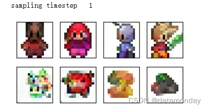
使用完全随机的上下文
# visualize samples with randomly selected context
plt.clf()
ctx = F.one_hot(torch.randint(0, 5, (32,)), 5).to(device=device).float()
samples, intermediate = sample_ddpm_context(32, ctx)
animation_ddpm_context = plot_sample(intermediate,32,4,save_dir, "ani_run", None, save=False)
HTML(animation_ddpm_context.to_jshtml())

def show_images(imgs, nrow=2):
    _, axs = plt.subplots(nrow, imgs.shape[0] // nrow, figsize=(4,2 ))
    axs = axs.flatten()
    for img, ax in zip(imgs, axs):
        img = (img.permute(1, 2, 0).clip(-1, 1).detach().cpu().numpy() + 1) / 2
        ax.set_xticks([])
        ax.set_yticks([])
        ax.imshow(img)
    plt.show()
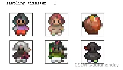
# user defined context
ctx = torch.tensor([
    # hero, non-hero, food, spell, side-facing
    [1,0,0,0,0],
    [1,0,0,0,0],
    [0,0,0,0,1],
    [0,0,0,0,1],
    [0,1,0,0,0],
    [0,1,0,0,0],
    [0,0,1,0,0],
    [0,0,1,0,0],
]).float().to(device)
samples, _ = sample_ddpm_context(ctx.shape[0], ctx)
show_images(samples)
通过浮点数来控制各种图片的混合效果
# mix of defined context
ctx = torch.tensor([
    # hero, non-hero, food, spell, side-facing
    [1,0,0,0,0],      #human
    [1,0,0.6,0,0],
    [0,0,0.6,0.4,0],
    [1,0,0,0,1],
    [1,1,0,0,0],
    [1,0,0,1,0]
]).float().to(device)
samples, _ = sample_ddpm_context(ctx.shape[0], ctx)
show_images(samples)
7. Speeding up
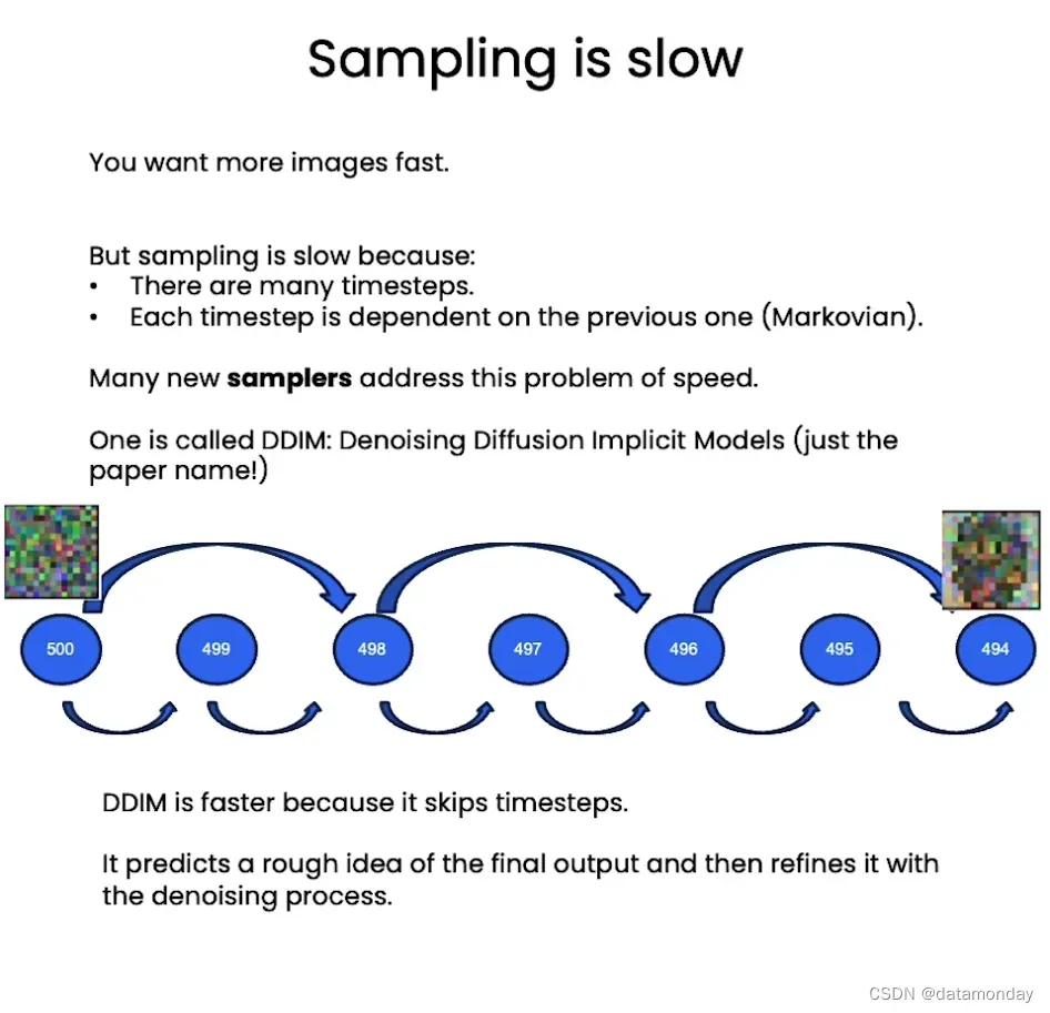
本小节将会介绍一种新的采样方法——DDIM,速度比DDPM快10倍以上。
训练NN的目标是想要快速地获得更多的图片。但是目前采样速度很慢,因为涉及到很多时间步骤,之前的例子中都是需要500步,才能得到一个好的样本。而且每个时间步都依赖与前一个时间步,它遵循马尔科夫链过程。幸运的是,有许多新的采样器可以解决这个问题,毕竟这一直是扩散模型的痛点。
去噪扩散隐式模型(Denoising Diffusion Implicit Models,DDIM)就是其中之一。
DDIM更快的原因是它能够跨过时间步长,而不再遵循马尔科夫假设。马尔科夫链实际上只适用于概率过程,但是DDIM从采样过程中去处了随机性,因此是确定性的。DDIM所做的本质上就是预测最终输出的粗略草图,然后用去噪过程对其进行细化。
下面是两个模型的对比:

# construct DDPM noise schedule
b_t = (beta2 - beta1) * torch.linspace(0, 1, timesteps + 1, device=device) + beta1
a_t = 1 - b_t
ab_t = torch.cumsum(a_t.log(), dim=0).exp()
ab_t[0] = 1

# construct model
nn_model = ContextUnet(in_channels=3, n_feat=n_feat, n_cfeat=n_cfeat, height=height).to(device)
# define sampling function for DDIM
# removes the noise using ddim
def denoise_ddim(x, t, t_prev, pred_noise):
    ab = ab_t[t]
    ab_prev = ab_t[t_prev]

    x0_pred = ab_prev.sqrt() / ab.sqrt() * (x - (1 - ab).sqrt() * pred_noise)
    dir_xt = (1 - ab_prev).sqrt() * pred_noise

    return x0_pred + dir_xt
# load in model weights and set to eval mode
nn_model.load_state_dict(torch.load(f"{save_dir}/model_31.pth", map_location=device))
nn_model.eval()
print("Loaded in Model without context")
# sample quickly using DDIM
@torch.no_grad()
def sample_ddim(n_sample, n=20):
    # x_T ~ N(0, 1), sample initial noise
    samples = torch.randn(n_sample, 3, height, height).to(device)

    # array to keep track of generated steps for plotting
    intermediate = []
    step_size = timesteps // n
    for i in range(timesteps, 0, -step_size):
        print(f'sampling timestep {i:3d}', end='\r')

        # reshape time tensor
        t = torch.tensor([i / timesteps])[:, None, None, None].to(device)

        eps = nn_model(samples, t)    # predict noise e_(x_t,t)
        samples = denoise_ddim(samples, i, i - step_size, eps)
        intermediate.append(samples.detach().cpu().numpy())

    intermediate = np.stack(intermediate)
    return samples, intermediate
不带上下文的DDIM生成样例
# visualize samples
plt.clf()
samples, intermediate = sample_ddim(32, n=25)

animation_ddim = plot_sample(intermediate,32,4,save_dir, "ani_run", None, save=False)

HTML(animation_ddim.to_jshtml())

# load in model weights and set to eval mode
nn_model.load_state_dict(torch.load(f"{save_dir}/context_model_31.pth", map_location=device))
nn_model.eval()
print("Loaded in Context Model")
# fast sampling algorithm with context
@torch.no_grad()
def sample_ddim_context(n_sample, context, n=20):
    # x_T ~ N(0, 1), sample initial noise
    samples = torch.randn(n_sample, 3, height, height).to(device)

    # array to keep track of generated steps for plotting
    intermediate = []
    step_size = timesteps // n
    for i in range(timesteps, 0, -step_size):
        print(f'sampling timestep {i:3d}', end='\r')

        # reshape time tensor
        t = torch.tensor([i / timesteps])[:, None, None, None].to(device)

        eps = nn_model(samples, t, c=context)    # predict noise e_(x_t,t)
        samples = denoise_ddim(samples, i, i - step_size, eps)
        intermediate.append(samples.detach().cpu().numpy())

    intermediate = np.stack(intermediate)
    return samples, intermediate
带上下文的DDIM生成样例
# visualize samples
plt.clf()
ctx = F.one_hot(torch.randint(0, 5, (32,)), 5).to(device=device).float()
samples, intermediate = sample_ddim_context(32, ctx)

animation_ddpm_context = plot_sample(intermediate,32,4,save_dir, "ani_run", None, save=False)

HTML(animation_ddpm_context.to_jshtml())

速度对比
# helper function; removes the predicted noise (but adds some noise back in to avoid collapse)
def denoise_add_noise(x, t, pred_noise, z=None):
    if z is None:
        z = torch.randn_like(x)
    noise = b_t.sqrt()[t] * z
    mean = (x - pred_noise * ((1 - a_t[t]) / (1 - ab_t[t]).sqrt())) / a_t[t].sqrt()
    return mean + noise
# sample using standard algorithm
@torch.no_grad()
def sample_ddpm(n_sample, save_rate=20):
    # x_T ~ N(0, 1), sample initial noise
    samples = torch.randn(n_sample, 3, height, height).to(device)

    # array to keep track of generated steps for plotting
    intermediate = []
    for i in range(timesteps, 0, -1):
        print(f'sampling timestep {i:3d}', end='\r')

        # reshape time tensor
        t = torch.tensor([i / timesteps])[:, None, None, None].to(device)

        # sample some random noise to inject back in. For i = 1, don't add back in noise
        z = torch.randn_like(samples) if i > 1 else 0

        eps = nn_model(samples, t)    # predict noise e_(x_t,t)
        samples = denoise_add_noise(samples, i, eps, z)
        if i % save_rate ==0 or i==timesteps or i<8:
            intermediate.append(samples.detach().cpu().numpy())

    intermediate = np.stack(intermediate)
    return samples, intermediate
%timeit -r 1 sample_ddim(32, n=25)
%timeit -r 1 sample_ddpm(32, )
6 s ± 0 ns per loop (mean ± std. dev. of 1 run, 1 loop each)
1min 58s ± 0 ns per loop (mean ± std. dev. of 1 run, 1 loop each)
采样如果在500步以上,DDPM效果会更好,500步以内,DDIM会更好。
8. Summary
扩散模型不仅仅可以用于图片,还可以通过Prompt,让它用于文本反演(textual inversion),图像修复,音乐生成,视频生成,药物发现等。
Stable Diffusion 采用一种名为潜在扩散(latent diffusion)的方法,它直接在图像嵌入(Embedding)上操作,而不是在图像上操作,使得过程更加高效。此外还有一些方法值得尝试,交叉注意力文本调节(cross-attention text conditioning),无分类器引导(classifier-free guidance)等。
扩散模型,去噪,采样,DDPM,DDIM,U-Net,上下文融入模型。
samples, i, eps, z)
if i % save_rate 0 or itimesteps or i<8:
intermediate.append(samples.detach().cpu().numpy())
intermediate = np.stack(intermediate)
return samples, intermediate
```python
%timeit -r 1 sample_ddim(32, n=25)
%timeit -r 1 sample_ddpm(32, )
6 s ± 0 ns per loop (mean ± std. dev. of 1 run, 1 loop each)
1min 58s ± 0 ns per loop (mean ± std. dev. of 1 run, 1 loop each)
采样如果在500步以上,DDPM效果会更好,500步以内,DDIM会更好。
8. Summary
扩散模型不仅仅可以用于图片,还可以通过Prompt,让它用于文本反演(textual inversion),图像修复,音乐生成,视频生成,药物发现等。
Stable Diffusion 采用一种名为潜在扩散(latent diffusion)的方法,它直接在图像嵌入(Embedding)上操作,而不是在图像上操作,使得过程更加高效。此外还有一些方法值得尝试,交叉注意力文本调节(cross-attention text conditioning),无分类器引导(classifier-free guidance)等。
文章出处登录后可见!