大家好,我是带我去滑雪!
本期为大家介绍决策树算法,它一种基学习器,广泛应用于集成学习,用于大幅度提高模型的预测准确率。决策树在分区域时,会考虑特征向量对响应变量的影响,且每次仅使用一个分裂变量,这使得决策树很容易应用于高维空间,且不受噪声变量的影响。这是因为如果特征向量包含噪声变量(对响应变量无作用的变量),那么该特征向量将不会被选为分裂变量,故不影响决策树的建模。在某种意义上,决策树的分区预测更具智慧,可视为自适应邻近法。如果将决策树用于分类问题,则称为分类决策树,如果将决策树用于回归问题,则称为回归决策树。下面介绍两个python案例,练习实操。
目录
1、分类决策树案例
(1)导入相关模块与数据
(2)数据清洗与划分训练集、测试集
(3)构建决策树
(4)考察成本复杂性参数与叶节点总不纯度的关系
(5)通过10折交叉验证选择最优的超参数ccp_alpha值,并拟合模型
(6)计算每个变量重要性并进行可视化
(7)使用测试集进行预测,并计算混淆矩阵
(8)计算预测准确率与灵敏度、kappa指标
(9)以0.1作为临界值重新进行预测,计算混淆矩阵与预测准确率、灵敏度
2、回归决策树案例
(1)导入数据与相应模块
(2)划分训练集和测试集,构建决策树模型,并绘制决策树
(3)考察成本复杂性超参数与叶节点总均方误差的关系
(4)通过10折交叉验证选择最优超参数alpha值,并以此构建决策树模型,绘制决策树
(5)计算各变量的重要性值,并进行可视化
(6)使用测试集进行预测,画出预测值与实际值的散点图
1、分类决策树案例
使用葡萄牙银行市场营销的数据集bank-additional.csv来进行分类决策树操作,该数据集的特征变量包括客户的年龄(age)、职业类型(job)、婚姻状况(marital)、受教育程度(education)、是否信用违约(default)、是否有房贷(housing)、是否有个人贷款(loan)、工作单位人数(nr.employed)、消费者信心指数(cons.conf.indx)等共计20个,响应变量y为二分类变量,表示在接到银行的直销电话后,客户是否会购买银行定期存款产品。
(1)导入相关模块与数据
import numpy as np
import pandas as pd
import matplotlib.pyplot as plt
from sklearn.model_selection import train_test_split
from sklearn.model_selection import KFold, StratifiedKFold
from sklearn.model_selection import GridSearchCV
from sklearn.tree import DecisionTreeRegressor,export_text
from sklearn.tree import DecisionTreeClassifier, plot_tree
from sklearn.metrics import cohen_kappa_score
bank = pd.read_csv(r”E:\工作\硕士\博客\博客28-分类决策树与回归决策树\bank-additional.csv”, sep=’;’)
bank.shape#考察数据框维度pd.options.display.max_columns = 30 #增大pandas数据框的最大显示列数
bank输出结果:
age job marital education default housing loan contact month day_of_week duration campaign pdays previous poutcome emp.var.rate cons.price.idx cons.conf.idx euribor3m nr.employed y 0 30 blue-collar married basic.9y no yes no cellular may fri 487 2 999 0 nonexistent -1.8 92.893 -46.2 1.313 5099.1 no 1 39 services single high.school no no no telephone may fri 346 4 999 0 nonexistent 1.1 93.994 -36.4 4.855 5191.0 no 2 25 services married high.school no yes no telephone jun wed 227 1 999 0 nonexistent 1.4 94.465 -41.8 4.962 5228.1 no 3 38 services married basic.9y no unknown unknown telephone jun fri 17 3 999 0 nonexistent 1.4 94.465 -41.8 4.959 5228.1 no 4 47 admin. married university.degree no yes no cellular nov mon 58 1 999 0 nonexistent -0.1 93.200 -42.0 4.191 5195.8 no … … … … … … … … … … … … … … … … … … … … … … 4114 30 admin. married basic.6y no yes yes cellular jul thu 53 1 999 0 nonexistent 1.4 93.918 -42.7 4.958 5228.1 no 4115 39 admin. married high.school no yes no telephone jul fri 219 1 999 0 nonexistent 1.4 93.918 -42.7 4.959 5228.1 no 4116 27 student single high.school no no no cellular may mon 64 2 999 1 failure -1.8 92.893 -46.2 1.354 5099.1 no 4117 58 admin. married high.school no no no cellular aug fri 528 1 999 0 nonexistent 1.4 93.444 -36.1 4.966 5228.1 no 4118 34 management single high.school no yes no cellular nov wed 175 1 999 0 nonexistent -0.1 93.200 -42.0 4.120 5195.8 no 4119 rows × 21 columns
(2)数据清洗与划分训练集、测试集
bank = bank.drop(‘duration’, axis=1)#使用drop()方法去除无效变量duration
X_raw = bank.iloc[:, :-1]#取出所有的特征变量,不含最后一列的响应变量
X = pd.get_dummies(X_raw)#对所有的特征变量中分类变量变为数值型的虚拟变量
X.head(2)#考察数据矩阵x的前两个观测值输出结果:
age campaign pdays previous emp.var.rate cons.price.idx cons.conf.idx euribor3m nr.employed job_admin. job_blue-collar job_entrepreneur job_housemaid job_management job_retired … month_jul month_jun month_mar month_may month_nov month_oct month_sep day_of_week_fri day_of_week_mon day_of_week_thu day_of_week_tue day_of_week_wed poutcome_failure poutcome_nonexistent poutcome_success 0 30 2 999 0 -1.8 92.893 -46.2 1.313 5099.1 0 1 0 0 0 0 … 0 0 0 1 0 0 0 1 0 0 0 0 0 1 0 1 39 4 999 0 1.1 93.994 -36.4 4.855 5191.0 0 0 0 0 0 0 … 0 0 0 1 0 0 0 1 0 0 0 0 0 1 0 2 rows × 62 columns
y = bank.iloc[:, -1]#取出响应变量并赋值为y
X_train, X_test, y_train, y_test = train_test_split(X, y, stratify=y, test_size=1000, random_state=1)#将随机保留1000个观测值作为测试集,剩余用于训练集
(3)构建决策树
model = DecisionTreeClassifier(max_depth=2, random_state=123)#使用sklearnDecisionTreeClassifier类构造决策树
model.fit(X_train, y_train)#拟合决策树
model.score(X_test, y_test)#模型评价输出结果:
0.904plot_tree(model, feature_names=X.columns, node_ids=True, rounded=True, precision=2)#画出决策树
plt.savefig(“squares0.png”,
bbox_inches =”tight”,
pad_inches = 1,
transparent = True,
facecolor =”w”,
edgecolor =’w’,
dpi=300,
orientation =’landscape’)输出结果:
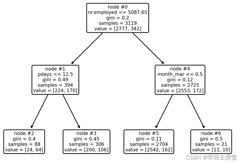
结果显示,测试集的预测准确率达到90.4%。
(4)考察成本复杂性参数与叶节点总不纯度的关系
model = DecisionTreeClassifier(random_state=123)
path = model.cost_complexity_pruning_path(X_train, y_train)#得到一系列ccp_alpha值与相应叶节点总不纯度
plt.plot(path.ccp_alphas, path.impurities, marker=’o’, drawstyle=’steps-post’,color=’pink’)#画图展示二者之间的关系
plt.xlabel(‘alpha (cost-complexity parameter)’)
plt.ylabel(‘Total Leaf Impurities’)
plt.title(‘Total Leaf Impurities vs alpha for Training Set’)
plt.savefig(“squares1.png”,
bbox_inches =”tight”,
pad_inches = 1,
transparent = True,
facecolor =”w”,
edgecolor =’w’,
dpi=300,
orientation =’landscape’)输出结果:
max(path.ccp_alphas), max(path.impurities)#寻找最大的ccp_alphas值与最大叶节点总不纯度值
输出结果:
(0.029949526543893212, 0.19525458100457016)
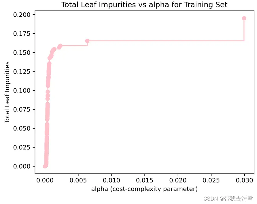
通过上图可以发现,当成本复杂性参数alpha为0时,并不惩罚决策树规模,导致每个观测值本身就为一个叶节点,总的叶节点的不纯度为0。当alpha上升时,对于决策树的惩罚力度增加,故叶节点总不纯度随之上升。当alpha的值约为0.02995时,决策树仅剩下树桩,叶节点总不纯度达到最大约为0.19525。
(5)通过10折交叉验证选择最优的超参数ccp_alpha值,并拟合模型
param_grid = {‘ccp_alpha’: path.ccp_alphas}#建立网格化
kfold = StratifiedKFold(n_splits=10, shuffle=True, random_state=1)#10折交叉验证选择最优超参数
model = GridSearchCV(DecisionTreeClassifier(random_state=123), param_grid, cv=kfold)
model.fit(X_train, y_train)
model.best_params_#获取最优超参数
model = model.best_estimator_#将模型重新定义为最优模型
model.score(X_test, y_test)#使用最优模型,计算测试集准确率
plot_tree(model, feature_names=X.columns, node_ids=True, impurity=True, proportion=True, rounded=True, precision=2)#proportion=True表示显示观测值的比重
plt.savefig(“squares2.png”,
bbox_inches =”tight”,
pad_inches = 1,
transparent = True,
facecolor =”w”,
edgecolor =’w’,
dpi=300,
orientation =’landscape’)输出结果:
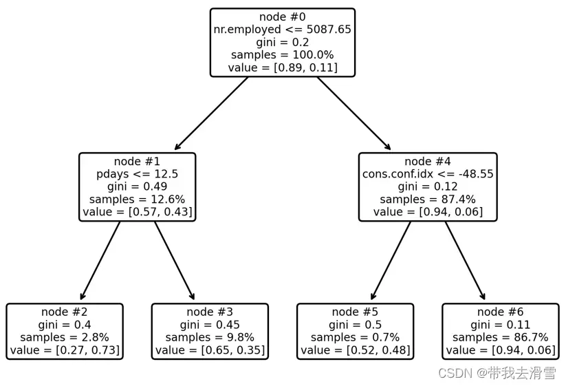
最优决策树解读:最优决策树只有4个终节点。其中根节点(node#0)拥有100%的样本数据,其中有购买意愿的有11%,没有购买意愿的为89%;从根节点出发,满足工作单位人数小于5088人的观测值进入左边的节点(node#1),反之进入右边的节点(node#4)。
节点node#1包含12.6%的样本数据,其中无购买意愿的比例为57%,而有购买意愿的比例为43%,从 节点node#1出发,满足条件自上次营销致电未过12.5天的观测值进入终结点node#2,反之进入node#3。在终节点node#2中有购买意愿的比例为73%,这意味着给当工作单位人数小于5088人且自上次营销致电未过12.5天的客户致电时,其购买存款理财产品的可能性最大。而node#3与node#5中有购买意愿的客户占比分别为35%、48%,也可以是致电的潜在客户人群。
(6)计算每个变量重要性并进行可视化
model.feature_importances_#计算每个变量的重要性值
sorted_index = model.feature_importances_.argsort()
plt.barh(range(X_train.shape[1]), model.feature_importances_[sorted_index])
plt.yticks(np.arange(X_train.shape[1]), X_train.columns[sorted_index])
plt.xlabel(‘Feature Importance’)
plt.ylabel(‘Feature’)
plt.title(‘Decision Tree’)
plt.tight_layout()
plt.savefig(“squares3.png”,
bbox_inches =”tight”,
pad_inches = 1,
transparent = True,
facecolor =”w”,
edgecolor =’w’,
dpi=300,
orientation =’landscape’)输出结果:
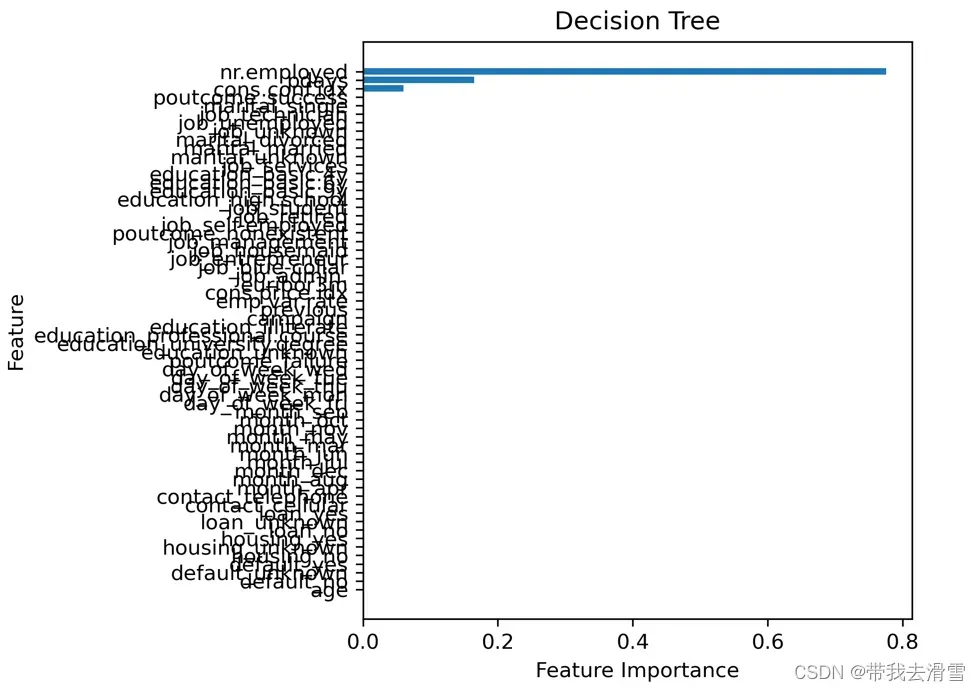
结果显示,只有三个变量的重要性值不为0,其他变量的重要性值均为0,这是因为在分裂决策树时,没有用到这些变量。
(7)使用测试集进行预测,并计算混淆矩阵
pred = model.predict(X_test)#使用测试集进行预测
table = pd.crosstab(y_test, pred, rownames=[‘Actual’], colnames=[‘Predicted’])#展示混淆矩阵
table输出结果:
Predicted no yes Actual no 880 11 yes 85 24
(8)计算预测准确率与灵敏度、kappa指标
table = np.array(table)
Accuracy = (table[0, 0] + table[1, 1]) / np.sum(table)#计算预测准确率
Accuracy
输出结果:0.904Sensitivity = table[1, 1] / (table[1, 0] + table[1, 1])#计算灵敏度
Sensitivity输出结果:
0.22018348623853212cohen_kappa_score(y_test, pred)#计算kappa值
输出结果:
0.2960328518002493
结果显示虽然预测准确率达到90.4%,但决策树算法的灵敏度只有22%,即只能成功识别22%有购买意愿的客户。科恩的kappa指标值约为0.296,介于0.2至0.4区间,说明预测值与实际值的一致性一般。
(9)以0.1作为临界值重新进行预测,计算混淆矩阵与预测准确率、灵敏度
prob = model.predict_proba(X_test)%计算测试集中每位个体有购买意愿的概率
prob
model.classes_#确认第1列与第2列的类别,第1列为无购买意愿的,第2列为有购买意愿的
prob_yes = prob[:, 1]
pred_new = (prob_yes >= 0.1)#以0.1作为临界值
pred_new
table = pd.crosstab(y_test, pred_new, rownames=[‘Actual’], colnames=[‘Predicted’])
table
table = np.array(table)
Accuracy = (table[0, 0] + table[1, 1]) / np.sum(table)
Accuracy输出结果:
0.88

Sensitivity  = table[1, 1] / (table[1, 0] + table[1, 1])
Sensitivity
输出结果:
0.5412844036697247
结果显示,以0.1作为预测临界值,虽然预测准确率略有下降,但灵敏度却升高至54.1%。
2、回归决策树案例
使用波士顿房价数据集boston_housing_data.csv,该数据集有城镇人均犯罪率(CRIM)、住宅用地所占比例(ZN)、城镇中非住宅用地所占比例(INDUS)等共计13个特征变量,响应变量为社区房价中位数(MEDV)。
(1)导入数据与相应模块
import numpy as np
import pandas as pd
import matplotlib.pyplot as plt
import seaborn as sns
from sklearn.model_selection import train_test_split
from sklearn.model_selection import KFold, StratifiedKFold
from sklearn.model_selection import GridSearchCV
from sklearn.tree import DecisionTreeRegressor,export_text
from sklearn.tree import DecisionTreeClassifier, plot_tree
from sklearn.metrics import cohen_kappa_score
Boston=pd.read_csv(r”E:\工作\硕士\博客\博客28-分类决策树与回归决策树\boston_housing_data.csv”)
Boston输出结果:
CRIM ZN INDUS CHAS NOX RM AGE DIS RAD TAX PIRATIO B LSTAT MEDV 0 0.00632 18.0 2.31 0.0 0.538 6.575 65.2 4.0900 1 296.0 15.3 396.90 4.98 24.0 1 0.02731 0.0 7.07 0.0 0.469 6.421 78.9 4.9671 2 242.0 17.8 396.90 9.14 21.6 2 0.02729 0.0 7.07 0.0 0.469 7.185 61.1 4.9671 2 242.0 17.8 392.83 4.03 34.7 3 0.03237 0.0 2.18 0.0 0.458 6.998 45.8 6.0622 3 222.0 18.7 394.63 2.94 33.4 4 0.06905 0.0 2.18 0.0 0.458 7.147 54.2 6.0622 3 222.0 18.7 396.90 5.33 36.2 … … … … … … … … … … … … … … … 501 0.06263 0.0 11.93 0.0 0.573 6.593 69.1 2.4786 1 273.0 21.0 391.99 9.67 22.4 502 0.04527 0.0 11.93 0.0 0.573 6.120 76.7 2.2875 1 273.0 21.0 396.90 9.08 20.6 503 0.06076 0.0 11.93 0.0 0.573 6.976 91.0 2.1675 1 273.0 21.0 396.90 5.64 23.9 504 0.10959 0.0 11.93 0.0 0.573 6.794 89.3 2.3889 1 273.0 21.0 393.45 6.48 22.0 505 0.04741 0.0 11.93 0.0 0.573 6.030 80.8 2.5050 1 273.0 21.0 396.90 7.88 11.9 506 rows × 14 columns
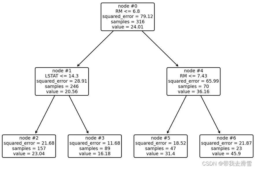
(2)划分训练集和测试集,构建决策树模型,并绘制决策树
data= Boston.iloc[:, :-1]#取出所有的特征变量,不含最后一列的响应变量
target=Boston.iloc[:, -1]#取出响应变量并赋值为target
Boston.feature_names=list(data.columns)#定义特征变量名称,方便后续绘制决策树
Boston.feature_names
X_train, X_test, y_train, y_test = train_test_split(data,target, test_size=0.3, random_state=0)#划分测试集和训练集
model = DecisionTreeRegressor(max_depth=2, random_state=123)#构建决策树
model.fit(X_train, y_train)#模型拟合
model.score(X_test, y_test)#求模型得分
print(export_text(model,feature_names=list(Boston.feature_names)))#输出决策树
plot_tree(model, feature_names=Boston.feature_names, node_ids=True, rounded=True, precision=2)#绘制决策树
plt.tight_layout()#将终节点在决策树中分开
plt.savefig(“squares4.png”,
bbox_inches =”tight”,
pad_inches = 1,
transparent = True,
facecolor =”w”,
edgecolor =’w’,
dpi=300,
orientation =’landscape’)输出结果:
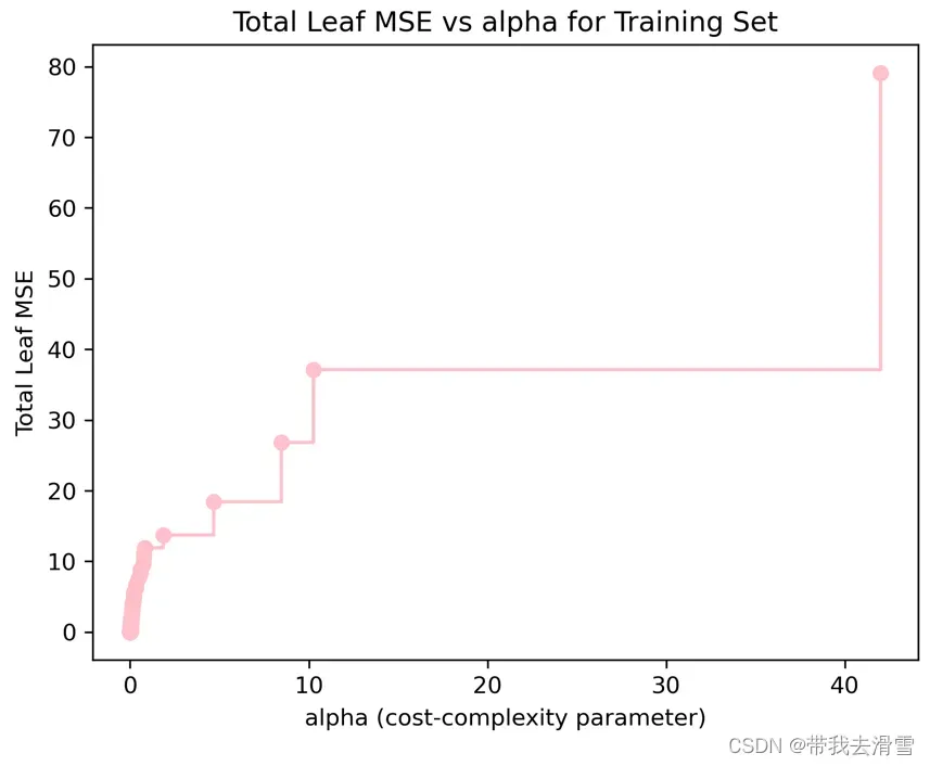
(3)考察成本复杂性超参数与叶节点总均方误差的关系
model = DecisionTreeRegressor(random_state=123)
path = model.cost_complexity_pruning_path(X_train, y_train)
plt.plot(path.ccp_alphas, path.impurities, marker=’o’, drawstyle=’steps-post’,color=’pink’)
plt.xlabel(‘alpha (cost-complexity parameter)’)
plt.ylabel(‘Total Leaf MSE’)
plt.title(‘Total Leaf MSE vs alpha for Training Set’)
plt.savefig(“squares5.png”,
bbox_inches =”tight”,
pad_inches = 1,
transparent = True,
facecolor =”w”,
edgecolor =’w’,
dpi=300,
orientation =’landscape’)
max(path.ccp_alphas), max(path.impurities)输出结果:
(41.99790024501699, 79.12414356673514)
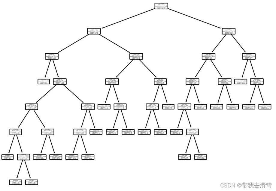
(4)通过10折交叉验证选择最优超参数alpha值,并以此构建决策树模型,绘制决策树
param_grid = {‘ccp_alpha’: path.ccp_alphas}
kfold = KFold(n_splits=10, shuffle=True, random_state=1)
model = GridSearchCV(DecisionTreeRegressor(random_state=123), param_grid, cv=kfold)
model.fit(X_train, y_train)
model.best_params_
model = model.best_estimator_
model.score(X_test,y_test)
plot_tree(model, feature_names=Boston.feature_names, node_ids=True, rounded=True, precision=2)
plt.tight_layout()
plt.savefig(“squares6.png”,
bbox_inches =”tight”,
pad_inches = 1,
transparent = True,
facecolor =”w”,
edgecolor =’w’,
dpi=300,
orientation =’landscape’)输出结果:
(5)计算各变量的重要性值,并进行可视化
model.feature_importances_
sorted_index = model.feature_importances_.argsort()
X = pd.DataFrame(data, columns=Boston.feature_names)
plt.barh(range(X.shape[1]), model.feature_importances_[sorted_index],color=’pink’,edgecolor=’red’)
plt.yticks(np.arange(X.shape[1]), X.columns[sorted_index])
plt.xlabel(‘Feature Importance’)
plt.ylabel(‘Feature’)
plt.title(‘Decision Tree’)
plt.tight_layout()
plt.savefig(“squares7.png”,
bbox_inches =”tight”,
pad_inches = 1,
transparent = True,
facecolor =”w”,
edgecolor =’w’,
dpi=300,
orientation =’landscape’)输出结果:
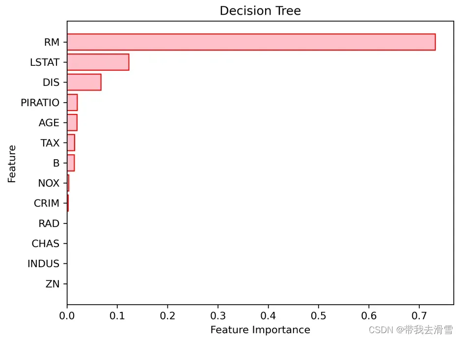
可以发现,变量房间数(RM)最为重要,其次是低端人口比重(LSTAT),再次为犯罪率(CRIM),最后是离就业中心距离(DIS)与反映社区的生师比(PTRATIO)。
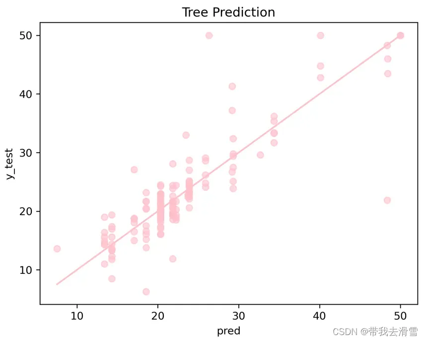
(6)使用测试集进行预测,画出预测值与实际值的散点图
pred = model.predict(X_test)
plt.scatter(pred, y_test, alpha=0.6,color=’pink’)
w = np.linspace(min(pred), max(pred), 100)
plt.plot(w, w,color=’pink’)
plt.xlabel(‘pred’)
plt.ylabel(‘y_test’)
plt.title(‘Tree Prediction’)
plt.savefig(“squares8.png”,
bbox_inches =”tight”,
pad_inches = 1,
transparent = True,
facecolor =”w”,
edgecolor =’w’,
dpi=300,
orientation =’landscape’)输出结果:
需要数据集的家人们可以去百度网盘(永久有效)获取:
链接:https://pan.baidu.com/s/173deLlgLYUz789M3KHYw-Q?pwd=0ly6
提取码:2138
更多优质内容持续发布中,请移步主页查看。
若有问题可邮箱联系:1736732074@qq.com
博主的WeChat:TCB1736732074
点赞+关注,下次不迷路!
版权声明:本文为博主作者:带我去滑雪原创文章,版权归属原作者,如果侵权,请联系我们删除!
原文链接:https://blog.csdn.net/qq_45856698/article/details/130463458