文章目录

• 一、集成学习概述
• 二、Bagging模型
• • 2.1 随机森林
  • • 2.1.1 随机森林介绍
    • 2.2.1 随机森林优势
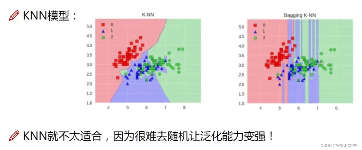
  • 2.2 KNN
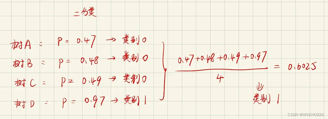
  • 2.3 软投票
  • 2.4 硬投票
  • 2.5 Bagging模型实战
  • • 2.5.1 构建实验数据集
    • 2.5.2 硬投票和软投票效果对比
    • • 2.5.2.1 硬投票效果
      • 2.5.2.2 软投票效果
    • 2.5.3 Bagging策略效果
    • • 2.5.3.1 用Bagging
      • 2.5.3.2 不用Bagging
    • 2.5.4 集成效果展示分析
    • 2.5.5 OOB袋外数据的作用
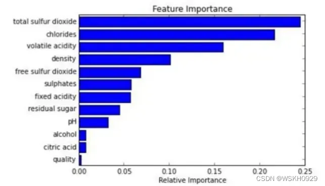
    • 2.5.6 特征重要性热度图展示
• 三、Boosting模型
• • 3.1 AdaBoost
  • • 3.1.1 AdaBoost算法概述
    • 3.1.2 SVM作为基本分类器实现AdaBoost
    • 3.1.3 Sklearn实现AdaBoost
  • 3.2 Gradient Boosting（GBDT）
  • • 3.2.1 用代码体会GBDT思想
    • 3.2.3 Sklearn实现GBDT
    • 3.2.3 提前停止策略
    • 3.2.4 停止方案实施
• 四、Stacking模型
• • 4.1 Stacking模型简介
  • 4.2 代码体会Stacking模型思想

一、集成学习概述

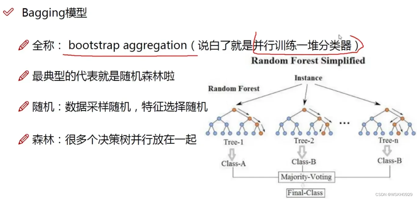
二、Bagging模型

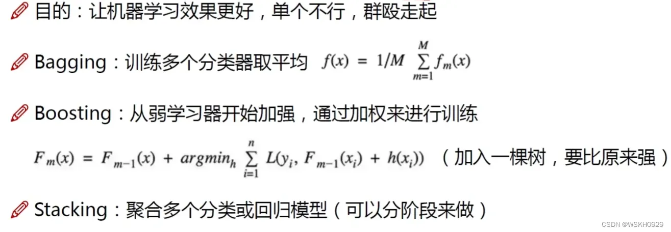
Bagging模型：并行训练一堆分类器，然后对所有分类器的结果求平均作为最后的结果

2.1 随机森林

2.1.1 随机森林介绍

Bagging模型中最典型的代表是：随机森林
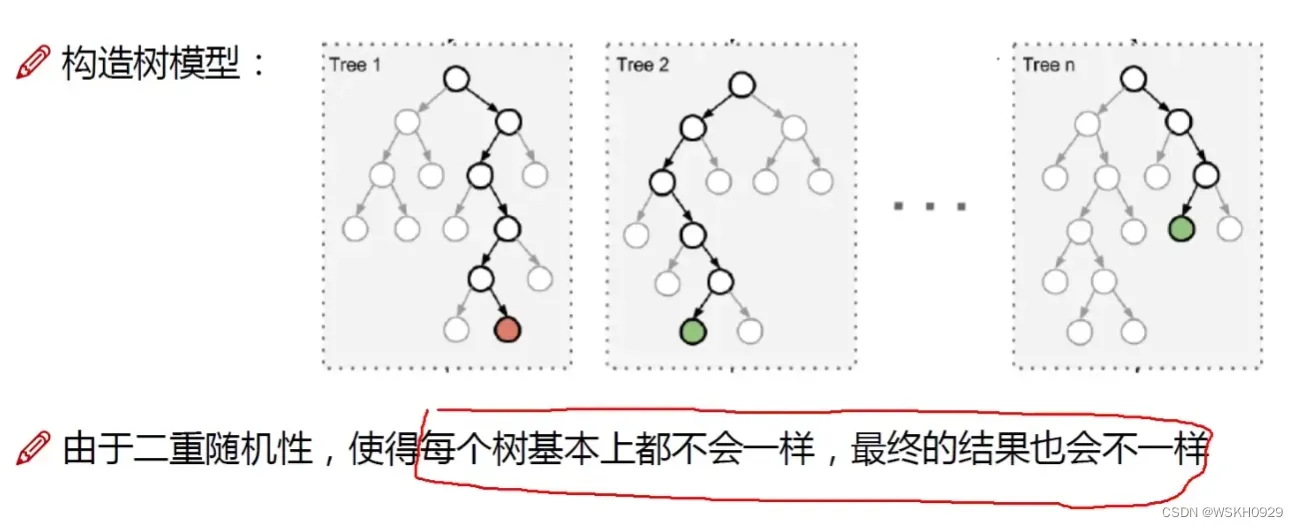
随机：数据随机采样，特征选择随机
森林：多个决策树并行放在一起

2.2.1 随机森林优势

• 能够处理高维度数据，并且不用做特征选择
• 训练完后，它能够给出哪些特征比较重要
• 容易并行化，速度较快
• 可以进行可视化展示，方便分析
  

2.2 KNN

2.3 软投票

加权平均

2.4 硬投票

少数服从多数

2.5 Bagging模型实战

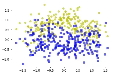
2.5.1 构建实验数据集

from sklearn.model_selection import train_test_split
from sklearn.datasets import make_moons
import matplotlib.pyplot as plt

X, y = make_moons(n_samples=500, noise=0.30, random_state=42)
X_train, X_test, y_train, y_test = train_test_split(X, y, random_state=42)

plt.plot(X[:, 0][y == 0], X[:, 1][y == 0], 'yo', alpha=0.6)
plt.plot(X[:, 0][y == 0], X[:, 1][y == 1], 'bs', alpha=0.6)

2.5.2 硬投票和软投票效果对比

2.5.2.1 硬投票效果

from sklearn.ensemble import RandomForestClassifier, VotingClassifier
from sklearn.linear_model import LogisticRegression
from sklearn.svm import SVC
from sklearn.metrics import accuracy_score

log_clf = LogisticRegression(random_state=520)
rnd_clf = RandomForestClassifier(random_state=520)
svm_clf = SVC(random_state=520)

voting_clf = VotingClassifier(estimators=[('lr', log_clf), ('rf', rnd_clf),
                                          ('svc', svm_clf)],
                              voting='hard')

for clf in (log_clf, rnd_clf, svm_clf, voting_clf):
    clf.fit(X_train, y_train)
    y_pred = clf.predict(X_test)
    print(clf.__class__.__name__, accuracy_score(y_test, y_pred))

输出：

LogisticRegression 0.864
RandomForestClassifier 0.872
SVC 0.896
VotingClassifier 0.888

2.5.2.2 软投票效果

from sklearn.ensemble import RandomForestClassifier, VotingClassifier
from sklearn.linear_model import LogisticRegression
from sklearn.svm import SVC
from sklearn.metrics import accuracy_score

log_clf = LogisticRegression(random_state=520)
rnd_clf = RandomForestClassifier(random_state=520)
svm_clf = SVC(random_state=520,probability=True)

voting_clf = VotingClassifier(estimators=[('lr', log_clf), ('rf', rnd_clf),
                                          ('svc', svm_clf)],
                              voting='soft')

for clf in (log_clf, rnd_clf, svm_clf, voting_clf):
    clf.fit(X_train, y_train)
    y_pred = clf.predict(X_test)
    print(clf.__class__.__name__, accuracy_score(y_test, y_pred))

输出：

LogisticRegression 0.864
RandomForestClassifier 0.872
SVC 0.896
VotingClassifier 0.912

结论：软投票比硬投票更靠谱一些

2.5.3 Bagging策略效果

2.5.3.1 用Bagging

from sklearn.ensemble import BaggingClassifier
from sklearn.tree import DecisionTreeClassifier

bag_clf = BaggingClassifier(DecisionTreeClassifier(),
                            n_estimators=500,
                            max_samples=100,
                            bootstrap=True,
                            n_jobs=-1,
                            random_state=520)
bag_clf.fit(X_train, y_train)
y_pred = bag_clf.predict(X_test)
print(accuracy_score(y_test, y_pred))

输出：

0.904

2.5.3.2 不用Bagging

tree_clf = DecisionTreeClassifier(random_state=42)
tree_clf.fit(X_train, y_train)
y_pred_tree = tree_clf.predict(X_test)
print(accuracy_score(y_test, y_pred_tree))

输出：

0.856

结论：用Bagging策略的预测效果更好

2.5.4 集成效果展示分析

from matplotlib.colors import ListedColormap


def plot_decision_boundary(clf,
                           X,
                           y,
                           axes=[-1.5, 2.5, -1, 1.5],
                           alpha=0.5,
                           contour=True):
    x1s = np.linspace(axes[0], axes[1], 100)
    x2s = np.linspace(axes[2], axes[3], 100)
    x1, x2 = np.meshgrid(x1s, x2s)
    X_new = np.c_[x1.ravel(), x2.ravel()]
    y_pred = clf.predict(X_new).reshape(x1.shape)
    custom_cmap = ListedColormap(['#fafab0', '#9898ff', '#a0faa0'])
    plt.contourf(x1,x2,y_pred,cmap=custom_cmap,alpha=0.3)
    if contour:
        custom_cmap2 = ListedColormap(['#7d7d58', '#4c4c7f', '#507d50'])
        plt.contour(x1, x2, y_pred)
    plt.plot(X[:, 0][y == 0], X[:, 1][y == 0], 'yo', alpha=0.6)
    plt.plot(X[:, 0][y == 0], X[:, 1][y == 1], 'bs', alpha=0.6)
    plt.axis(axes)
    plt.xlabel('x1')
    plt.xlabel('x2')

plt.figure(figsize=(12, 5))
plt.subplot(121)
plot_decision_boundary(tree_clf, X, y)
plt.title('Decision Tree')
plt.subplot(122)
plot_decision_boundary(bag_clf, X, y)
plt.title('Decision Tree With Bagging')

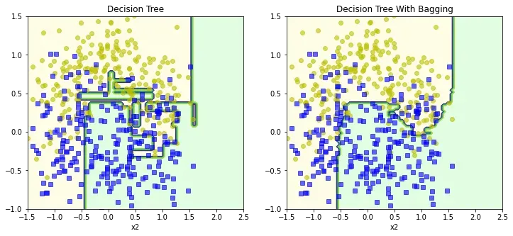
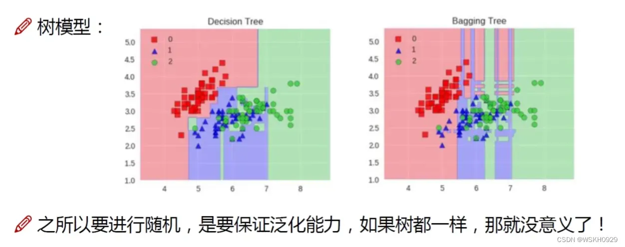
结论：采用Bagging策略的模型过拟合风险更小

2.5.5 OOB袋外数据的作用

bag_clf = BaggingClassifier(DecisionTreeClassifier(),
                            n_estimators=500,
                            max_samples=100,
                            bootstrap=True,
                            n_jobs=-1,
                            random_state=42,
                            oob_score=True)
bag_clf.fit(X_train, y_train)
print(bag_clf.oob_score_)

输出：

0.9253333333333333

y_pred = bag_clf.predict(X_test)
print(accuracy_score(y_test, y_pred))

输出：

0.904

结论：OOB袋外数据可以作为验证集对模型进行准确率的计算，比测试集计算的准确率略高，但相差不多

2.5.6 特征重要性热度图展示

from sklearn.datasets import load_iris

iris = load_iris()
rf_clf = RandomForestClassifier(n_estimators=500, n_jobs=-1)
rf_clf.fit(iris['data'], iris['target'])
for name, score in zip(iris['feature_names'], rf_clf.feature_importances_):
    print(name, score)

输出：

sepal length (cm) 0.09370373939142465
sepal width (cm) 0.022001401734976455
petal length (cm) 0.4505649464716102
petal width (cm) 0.4337299124019887

from sklearn.datasets import fetch_openml
import matplotlib
mnist = fetch_openml('mnist_784')

def plot_digit(data):
    image = data.reshape(28, 28)
    plt.imshow(image, cmap=matplotlib.cm.hot)
    plt.axis('off')


rf_clf = RandomForestClassifier(n_estimators=500, n_jobs=-1)
rf_clf.fit(mnist['data'], mnist['target'])

plot_digit(rf_clf.feature_importances_)
char = plt.colorbar(ticks=[
    rf_clf.feature_importances_.min(),
    rf_clf.feature_importances_.max()
])
char.ax.set_yticklabels(['Not important', 'Very importang'])

输出：

结论：RF输出的特征重要性热度图表示（颜色越接近黑色表示特征越不重要），在手写数据集中，中间的像素（特征）较为重要

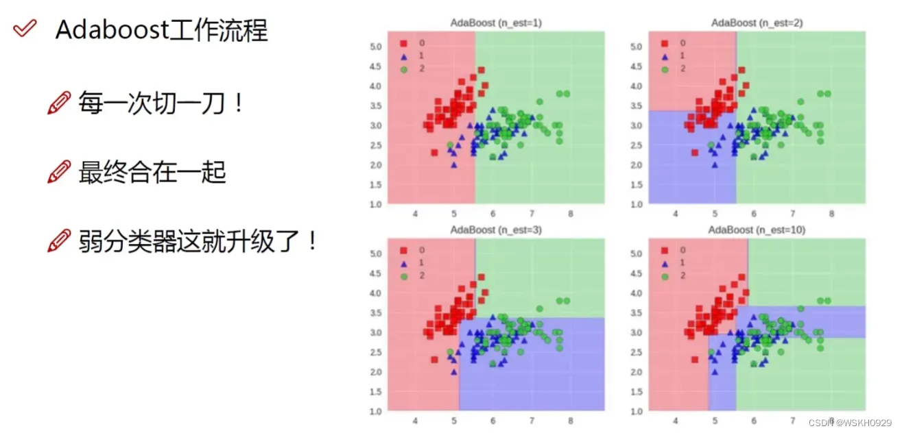
三、Boosting模型

典型代表：AdaBoost、Xgboost
AdaBoost会根据前一次的分类效果调整数据权重
解释：如果某一个数据在这次分错了，那么在下一次我就会给它更大的权重
最终的结果：每个分类器根据自身的准确性来确定各自的权重，再合体

3.1 AdaBoost

3.1.1 AdaBoost算法概述

跟上学考试一样，这次做错的题，需要额外注意，下次就不要做错了

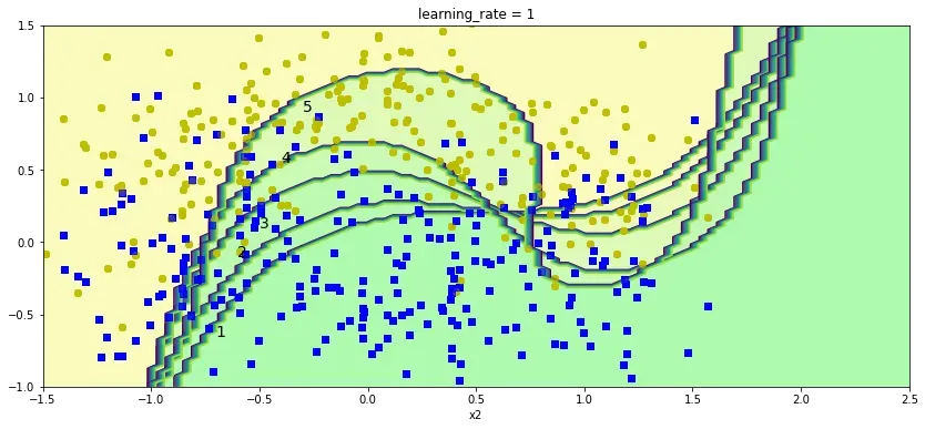
3.1.2 SVM作为基本分类器实现AdaBoost

plt.figure(figsize=(14, 6))
learning_rate = 1
sample_weights = np.ones(len(X_train))
for i in range(5):
    svm_clf = SVC(kernel='rbf', C=0.05, random_state=42)
    svm_clf.fit(X_train, y_train, sample_weight=sample_weights)
    y_pred = svm_clf.predict(X_train)
    sample_weights[y_pred != y_train] *= (1 + learning_rate)
    plot_decision_boundary(svm_clf, X, y, alpha=0.2)
    plt.title('learning_rate = {}'.format(learning_rate))
plt.text(-0.7, -0.65, "1", fontsize=14)
plt.text(-0.6, -0.10, "2", fontsize=14)
plt.text(-0.5, 0.10, "3", fontsize=14)
plt.text(-0.4, 0.55, "4", fontsize=14)
plt.text(-0.3, 0.90, "5", fontsize=14)
plt.show()

plt.figure(figsize=(14, 6))
learning_rate = 0.5
sample_weights = np.ones(len(X_train))
for i in range(5):
    svm_clf = SVC(kernel='rbf', C=0.05, random_state=42)
    svm_clf.fit(X_train, y_train, sample_weight=sample_weights)
    y_pred = svm_clf.predict(X_train)
    sample_weights[y_pred != y_train] *= (1 + learning_rate)
    plot_decision_boundary(svm_clf, X, y, alpha=0.2)
    plt.title('learning_rate = {}'.format(learning_rate))
plt.show()

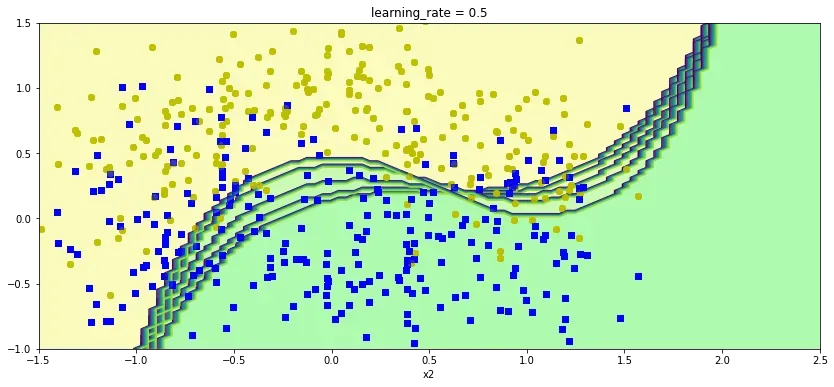
结论：AdaBoost中，学习率越大，每一步的更新就越快

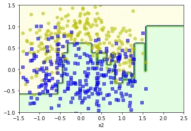
3.1.3 Sklearn实现AdaBoost

from sklearn.ensemble import AdaBoostClassifier

ada_clf = AdaBoostClassifier(DecisionTreeClassifier(max_depth=1),
                             n_estimators=200,
                             learning_rate=0.5,
                             random_state=42)
ada_clf.fit(X_train,y_train)
plot_decision_boundary (ada_clf,X,y)

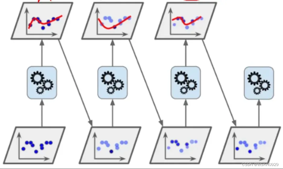
3.2 Gradient Boosting（GBDT）

GBDT中的代表模型：

• GDBT（第一代）
• XgBoost（第二代）
• LightGBM（第三代，效果通常最好）

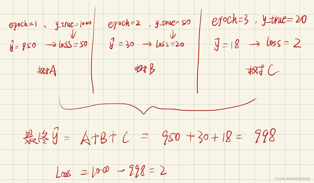
下图展现了GBDT的提升过程，通过不断加入树去弥补之前的Loss，使得模型整体预测效果得到提升：

3.2.1 用代码体会GBDT思想

# 导入库
from sklearn.tree import DecisionTreeRegressor
from sklearn.metrics import mean_absolute_error
# 构造测试数据
np.random.seed(42)
X = np.random.rand(100, 1) - 0.5
y = 3 * X[:, 0] * 2 + 0.05 * np.random.randn(100)
# 开始Gradient Boost循环
y_lst = [y]
tree_regl_lst = []
for i in range(10):
    # 实例化决策树回归器 max_depth=2 防止过拟合
    tree_regl = DecisionTreeRegressor(max_depth=2)
    tree_regl.fit(X,y_lst[i])
    y_hat = tree_regl.predict(X)
    print("MAE:",mean_absolute_error(y_lst[i],y_hat))
    y_lst.append(y_lst[i] - y_hat)
    tree_regl_lst.append(tree_regl)

输出：

MAE: 0.35567640260211664
MAE: 0.2757033790340715
MAE: 0.2220536712621441
MAE: 0.18640823041945379
MAE: 0.15983867589863676
MAE: 0.13915823769411198
MAE: 0.11948140923031975
MAE: 0.10646877400035713
MAE: 0.1036924652651969
MAE: 0.09089276292058762

结论：GDBT通过不断加入树，对上一次Loss进行再次训练，从而改进整体Loss

3.2.3 Sklearn实现GBDT

from sklearn.ensemble import GradientBoostingRegressor

gbrt = GradientBoostingRegressor(max_depth=2,
                                 n_estimators=3,
                                 learning_rate=1.0,
                                 random_state=41)
gbrt.fit(X, y)

3.2.3 提前停止策略

from sklearn.metrics import mean_squared_error

X_train, X_val, y_train, y_val = train_test_split(X, y, random_state=49)
gbrt = GradientBoostingRegressor(max_depth=2,
                                 n_estimators=120,
                                 random_state=42)
gbrt.fit(X_train, y_train)
errors = [
    mean_squared_error(y_val, y_pred) for y_pred in gbrt.staged_predict(X_val)
]
# 最佳迭代次数
bst_n_estimators = np.argmin(errors)
# 最小error
min_error = np.min(errors)

plt.figure(figsize = (11,4))
plt.plot (errors,'b.-')
plt.plot ([bst_n_estimators,bst_n_estimators],[0,min_error],'r--')
plt.plot ([0,120],[min_error,min_error],'r--')
plt.axis([0,120,0,0.01])
plt.title('Val Error')

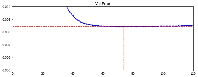
从上图可以看出，GBDT中不是加入树越多越好，在加入75个树往后，Error反而升高了，所以我们需要找到最佳树的个数，而不是一味地增加树的个数

3.2.4 停止方案实施

利用Sklearn提供的GBDT接口的热启动参数，使得模型每一次训练的信息得以保留，下一次可以接着训练
然后每次迭代判断当前损失是否提升，如果是则对error_going_up进行加1操作，当error_going_up达到一个阈值，则提前终止

# warm_start 热启动，保存上一次训练的信息，接着训练
gbrt = GradientBoostingRegressor(max_depth=2, random_state=42, warm_start=True)

error_going_up = 0
min_val_error = float('inf')
for n_estimators in range(1, 120):
    gbrt.n_estimators = n_estimators
    gbrt.fit(X_train, y_train)
    y_pred = gbrt.predict(X_val)
    val_error = mean_squared_error(y_val, y_pred)
    if val_error < min_val_error:
        min_val_error = val_error
        error_going_up = 0
    else:
        error_going_up += 1
        if error_going_up == 5:
            print("best_n_estimators:",n_estimators)
            break
print("min_val_error:",min_val_error)

输出：

best_n_estimators: 80
min_val_error: 0.00683519138553835

四、Stacking模型

4.1 Stacking模型简介

堆叠：很暴力，拿来一堆直接上（各种分类器都来了）
可以堆叠各种各样的分类器（KNN、SVM、RF、神经网络等等）
分阶段：第一阶段得出各自的结果，第二阶段再用前一阶段的结果训练
为了刷结果，不择手段！

4.2 代码体会Stacking模型思想

from sklearn.ensemble import RandomForestClassifier, ExtraTreesclassifier
from sklearn.svm import LinearSVC
from sklearn.neural_network import MLPClassifier

# 定义一阶段的4个分类器
random_forest_clf = RandomForestClassifier(random_state=42)
extra_trees_clf = ExtraTreesClassifier(random_state=42)
svm_clf = LinearSVC(random_state=42)
mlp_clf = MLPClassifier(random_state=42)
estimators = [random_forest_clf, extra_trees_clf, svm_clf, mlp_clf]

# 训练每个一阶段的分类器
for estimator in estimators:
    print("Training the",estimator)
    estimator.fit(X_train,y_train)

# 获取一阶段的输出结果
X_val_predictions = np.empty((len(X_val),len(estimators)),dtype=np.float32)
for index,estimator in enumerate(estimators):
    X_val_predictions[:,index]estimator.predict(X_val)
    
# 构造二阶段分类器
rnd_forest_blender = RandomForestClassifier(n_estimators=200,oob_score=True,random_state=42)

# 用一阶段的输出结果训练二阶段分类器
rnd_forest_blender.fit(X_val_predictions,y_val)