文章目录
- 1.导入库
- 2.引入机器学习的模型
- 2.1 逻辑回归模型
- 2.2 随机森林
- 2.3 支持向量机
- 2.4 K最近邻
- 2.5 决策树
- 3. 对数据处理
- 3.1 导入数据
- 3.2 处理训练集缺失值
- 3.2.1 查看维度
- 3.2.2 查看缺失的个数
- 3.2.3 处理缺失的上船港口(Embarked)
- 处理缺失的年龄(Age)
- 处理缺失的客舱号(Cabin)
- 3.3 对训练集的数据进行处理
- 3.3.1 打印前5行查看数据集
- 3.3.2 处理Pclass(客舱等级)
- 3.3.3 处理姓名
- 3.3.4 处理性别
- 3.3.5 处理年龄
- 3.3.6 处理家庭
- 3.3.7 处理船票和票价
- 3.3.8 处理上船港口
- 3.4 处理测试集
- 3.5 查看相关性
- 3.6 划分训练集和检验集
- 4. 训练模型
- 4.1 逻辑回归模型
- 4.2 随机森林
- 4.3 支持向量机
- 4.4 K最近邻
- 4.5 决策树
- 5.测试模型
- 5.1 逻辑回归模型
- 5.2 随机森林
- 5.3 支持向量机
- 5.4 K最近邻
- 5.5 决策树
- 5.6 5种模型对比
- 6. 预测模型
- 6.1 逻辑回归模型
- 6.2 随机森林
- 6.3 支持向量机
- 6.4 K最近邻
- 6.5 决策树
- 6.6 将上述结果交至kaggle进行评分
- 7. 完整代码
- 8. 总结
1.导入库
小编一般喜欢在在代码的刚开始便导入所有要使用的库,这样可以直观明了的将自己的思路展现出来,并且对代码的布局也更加美观。
下面是泰坦尼克号需要使用的库:
import numpy as np
import pandas as pd
import matplotlib.pyplot as plt
import seaborn as sns
import random
其中关于matplotlib,numpy,pandas工具的使用可以参考小编写的例外一篇博客
机器学习入门基本使用工具(保姆式教学):matplotlib,numpy,pandas这一篇就够了
这里是泰坦尼克号的数据集链接:https://pan.baidu.com/s/1C8mRRSkSdBsVRZ5zv_zCbA?pwd=w45i
提取码:w45i
2.引入机器学习的模型
这里导入5个模型,用来比较各种模型之间的差距
2.1 逻辑回归模型
from sklearn.linear_model import LogisticRegression
2.2 随机森林
from sklearn.ensemble import RandomForestClassifier
2.3 支持向量机
from sklearn.svm import SVC
2.4 K最近邻
from sklearn.neighbors import KNeighborsClassifier
2.5 决策树
from sklearn.tree import DecisionTreeClassifier
3. 对数据处理
3.1 导入数据
#训练数据集
train_data = pd.read_csv(r"D:\data\python\taitanic\train.csv")
#测试数据集
test_data = pd.read_csv(r"D:\data\python\taitanic\test.csv")
3.2 处理训练集缺失值
3.2.1 查看维度
>>>print('训练数据集:', train_data.shape, '测试数据集:', test_data.shape)
>训练数据集: (891, 12) 测试数据集: (418, 11)
3.2.2 查看缺失的个数
>>>train_data.isnull().sum()
>PassengerId      0
 Survived         0
 Pclass           0
 Name             0
 Sex              0
 Age            177
 SibSp            0
 Parch            0
 Ticket           0
 Fare             0
 Cabin          687
 Embarked         2
 dtype: int64
3.2.3 处理缺失的上船港口(Embarked)
查看上船港口数
>>>plt.figure(figsize=(10,5),dpi=100)
>>>train_data['Embarked'].value_counts().plot(kind='bar')
>>>plt.savefig(r"D:\data\python\exercise\test2\1.png")
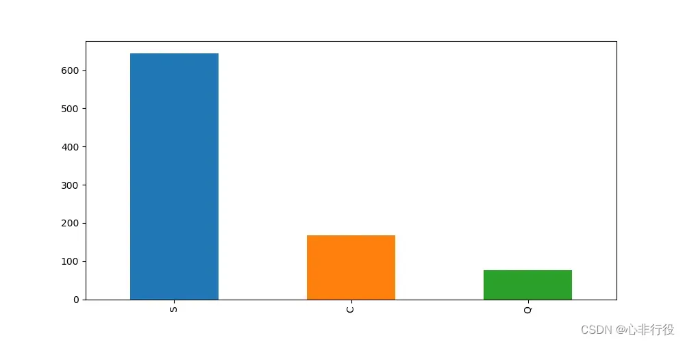
可以看到从S港口上船的人数最多,而数据只缺失两个,所以选取频率最高的填充到空白数据中
>>>train_data['Embarked'] = train_data['Embarked'].fillna('S')
>>>train_data.isnull().sum()
>PassengerId      0
 Survived         0
 Pclass           0
 Name             0
 Sex              0
 Age            177
 SibSp            0
 Parch            0
 Ticket           0
 Fare             0
 Cabin          687
 Embarked         0
 dtype: int64
处理缺失的年龄(Age)
处理空白年龄(Age),使用平均值填充
>>>train_data['Age'] = train_data['Age'].fillna(int(train_data['Age'].mean()))
>>>train_data.isnull().sum()
>PassengerId      0
 Survived         0
 Pclass           0
 Name             0
 Sex              0
 Age              0
 SibSp            0
 Parch            0
 Ticket           0
 Fare             0
 Cabin          687
 Embarked         0
 dtype: int64
处理缺失的客舱号(Cabin)
至此除了Cabin(船舱号)其他缺失值已经补充完毕.Cabin这一列数据值缺失过多选择填充会导致得到的数据过于片面,因此,选择删去这一列
>>>train_data.drop(columns = 'Cabin', axis=1,inplace=True)
>>>train_data.isnull().sum()
>PassengerId      0
 Survived         0
 Pclass           0
 Name             0
 Sex              0
 Age              0
 SibSp            0
 Parch            0
 Ticket           0
 Fare             0
 Embarked         0
 dtype: int64
至此,训练集的缺失值已经处理完毕
3.3 对训练集的数据进行处理
3.3.1 打印前5行查看数据集
>>>train_data.head()
>
	PassengerId	Survived	Pclass					Name								Sex		Age		SibSp	Parch	Ticket				Fare	Embarked
0	1			0			3		Braund, Mr. Owen Harris								male	22.0	1		0		A/5 21171			7.2500	S
1	2			1			1		Cumings, Mrs. John Bradley (Florence Briggs Th...	female	38.0	1		0		PC 17599			71.2833	C
2	3			1			3		Heikkinen, Miss. Laina								female	26.0	0		0		STON/O2. 3101282	7.9250	S
3	4			1			1		Futrelle, Mrs. Jacques Heath (Lily May Peel)		female	35.0	1		0		113803				53.1000	S
4	5			0			3		Allen, Mr. William Henry							male	35.0	0		0		373450				8.0500	S
3.3.2 处理Pclass(客舱等级)
使用get_dummies进行one-hot编码,列名前缀是Pclass
>>>pclassdf1 = pd.DataFrame()
>>>pclassdf1 = pd.get_dummies(train_data['Pclass'] , prefix='Pclass' )
>>>train_data = pd.concat([train_data, pclassdf1], axis=1)
>>>train_data.drop('Pclass',axis=1, inplace=True)
>>>train_data.head()
	PassengerId	Survived					Name								Sex		Age		SibSp	Parch	Ticket				Fare	Embarked	Pclass_1	Pclass_2	Pclass_3
0	1			0			Braund, Mr. Owen Harris								male	22.0	1		0		A/5 21171			7.2500	S			0			0			1
1	2			1			Cumings, Mrs. John Bradley (Florence Briggs Th...	female	38.0	1		0		PC 17599			71.2833	C			1			0			0
2	3			1			Heikkinen, Miss. Laina								female	26.0	0		0		STON/O2. 3101282	7.9250	S			0			0			1
3	4			1			Futrelle, Mrs. Jacques Heath (Lily May Peel)		female	35.0	1		0		113803				53.1000	S			1			0			0
4	5			0			Allen, Mr. William Henry							male	35.0	0		0		373450				8.0500	S			0			0			1
3.3.3 处理姓名
>>>def gettitle(name):
>>>    str1 = name.split(',')[1] #Mr. Owen Harris
>>>    str2 = str1.split('.')[0]#Mr
>>>    str3 = str2.strip()
>>>    return str3
#存放提取后的特征
>>>titledf1 = pd.DataFrame()
#map函数:对Series每个数据应用自定义的函数计算
>>>titledf1['Title'] = train_data['Name'].map(gettitle)
#查看titledf的种类
>>>titledf1['Title'].value_counts()
>Mr              517
 Miss            182
 Mrs             125
 Master           40
 Dr                7
 Rev               6
 Col               2
 Major             2
 Mlle              2
 Capt              1
 Lady              1
 Jonkheer          1
 Mme               1
 Sir               1
 the Countess      1
 Ms                1
 Don               1
 Name: Title, dtype: int64
#姓名中头衔字符串与定义头衔类别的对应关系
>>>title_mapdict = {
>>>                    "Capt":       "Officer",
>>>                    "Col":        "Officer",
>>>                    "Major":      "Officer",
>>>                    "Jonkheer":   "Royalty",
>>>                    "Don":        "Royalty",
>>>                    "Sir":        "Royalty",
>>>                    "Dr":         "Officer",
>>>                    "Rev":        "Officer",
>>>                    "the Countess":"Royalty",
>>>                    "Dona":       "Royalty",
>>>                    "Mme":        "Mrs",
>>>                    "Mlle":       "Miss",
>>>                    "Ms":         "Mrs",
>>>                    "Mr":         "Mr",
>>>                    "Mrs":        "Mrs",
>>>                    "Miss":       "Miss",
>>>                    "Master":     "Master",
>>>                    "Lady":       "Royalty"
>>>                    }
#map函数:对Series每个数据应用自定义的函数计算
>>>titledf1['Title'] = titledf1['Title'].map(title_mapdict)
#使用get_dummies进行one-hot编码
>>>titledf1 = pd.get_dummies(titledf1['Title'])
>>>train_data = pd.concat([train_data, titledf1], axis=1)
>>>train_data.drop('Name',axis=1, inplace=True)
>>>train_data.head()
>
	PassengerId	Survived	Sex		Age		SibSp	Parch	Ticket				Fare	Embarked	Pclass_1	Pclass_2	Pclass_3	Master	Miss	Mr	Mrs	Officer	Royalty
0	1			0			male	22.0	1		0		A/5 21171			7.2500	S			0			0			1			0		0		1	0	0		0
1	2	 		1			female	38.0	1		0		PC 17599			71.2833	C			1			0			0			0		0		0	1	0		0
2	3			1			female	26.0	0		0		STON/O2. 3101282	7.9250	S			0			0			1			0		1		0	0	0		0
3	4			1			female	35.0	1		0		113803				53.1000	S			1			0			0			0		0		0	1	0		0
4	5			0			male	35.0	0		0		373450				8.0500	S			0			0			1			0		0		1	0	0		0
3.3.4 处理性别
#处理性别
>>>sex_mapdict = {'male': 1, 'female': 0}
#map函数:对Series每个数据应用自定义的函数计算
>>>train_data['Sex'] = train_data['Sex'].map(sex_mapdict)
>>>sexdf1 = pd.DataFrame()
#使用get_dummies进行one-hot编码,产生虚拟变量(dummy variables),列名前缀是Sex
>>>sexdf1 = pd.get_dummies( train_data['Sex'], prefix='Sex')
>>>train_data = pd.concat([train_data, sexdf1], axis=1)
>>>train_data.drop('Sex',axis=1, inplace=True)
>>>train_data.head()
>

	PassengerId	Survived	Age		SibSp	Parch	Ticket				Fare	Embarked	Pclass_1	Pclass_2	Pclass_3	Master	Miss	Mr	Mrs	Officer	Royalty	Sex_0	Sex_1
0	1			0			22.0	1		0		A/5 21171			7.2500	S			0			0			1			0		0		1	0	0		0		0		1
1	2			1			38.0	1		0		PC 17599			71.2833	C			1			0			0			0		0		0	1	0		0		1		0
2	3			1			26.0	0		0		STON/O2. 3101282	7.9250	S			0			0			1			0		1		0	0	0		0		1		0
3	4			1			35.0	1		0		113803				53.1000	S			1			0			0			0		0		0	1	0		0		1		0
4	5			0			35.0	0		0		373450				8.0500	S			0			0			1			0		0		1	0	0		0		0		1
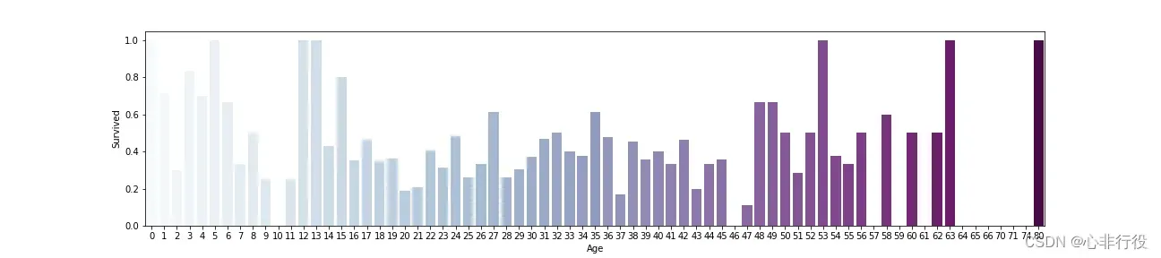
3.3.5 处理年龄
>>>plt.figure(figsize=(18,4))
>>>train_data['Age']=train_data['Age'].astype(np.int)
>>>average_age=train_data[['Age','Survived']].groupby('Age',as_index=False).mean()
>>>sns.barplot(x='Age',y='Survived',data=average_age,palette='BuPu')
>>>plt.savefig(r"D:\data\python\exercise\test2\2.png")
>>>agedf1 = pd.DataFrame(train_data['Age'])
>>>agedf1['Age_baby'] = agedf1['Age'].map(lambda s: 1 if 0 <= s < 15 else 0)
>>>agedf1['Age_youth'] = agedf1['Age'].map(lambda s: 1 if 15 <= s < 35 else 0)
>>>agedf1['Age_middle'] = agedf1['Age'].map(lambda s: 1 if 35 <= s <=60 else 0)
>>>agedf1['Age_old'] = agedf1['Age'].map(lambda s: 1 if 60 <= s else 0)
>>>train_data = pd.concat([train_data,agedf1], axis=1)
>>>train_data.drop('Age',axis=1, inplace=True)
>>>train_data.head()
>
	PassengerId	Survived	SibSp	Parch	Ticket				Fare	Embarked	Pclass_1	Pclass_2	Pclass_3	...	Mr	Mrs	Officer	Royalty	Sex_0	Sex_1	Age_baby	Age_youth	Age_middle	Age_old
0	1			0			1		0		A/5 21171			7.2500	S			0			0			1			...	1	0	0		0		0		1		0			1			0			0
1	2			1			1		0		PC 17599			71.2833	C			1			0			0			...	0	1	0		0		1		0		0			0			1			0
2	3			1			0		0		STON/O2. 3101282	7.9250	S			0			0			1			...	0	0	0		0		1		0		0			1			0			0
3	4			1			1		0		113803				53.1000	S			1			0			0			...	0	1	0		0		1		0		0			0			1			0
4	5			0			0		0		373450				8.0500	S			0			0			1			...	1	0	0		0		0		1		0			0			1			0
3.3.6 处理家庭
#存放家庭信息
>>>familydf1 = pd.DataFrame()
#家庭人数
>>>familydf1['FamilySize'] = train_data['Parch'] + train_data['SibSp'] + 1
#家庭类别
#if 条件为真的时候返回if前面内容,否则返回0
>>>familydf1['Family_Single'] = familydf1['FamilySize'].map(lambda s: 1 if s == 1 else 0)
>>>familydf1['Family_Small'] = familydf1['FamilySize'].map(lambda s: 1 if 2 <= s <= 4 else 0)
>>>familydf1['Family_Large'] = familydf1['FamilySize'].map(lambda s: 1 if 5 <= s else 0)
>>>familydf1.drop('FamilySize',axis=1, inplace=True)
>>>train_data = pd.concat([train_data, familydf1], axis=1)
>>>train_data.drop('Parch',axis=1, inplace=True)
>>>train_data.drop('SibSp',axis=1, inplace=True)
>>>train_data.head()
>
	PassengerId	Survived	Ticket				Fare	Embarked	Pclass_1	Pclass_2	Pclass_3	Master	Miss	...	Royalty	Sex_0	Sex_1	Age_baby	Age_youth	Age_middle	Age_old	Family_Single	Family_Small	Family_Large
0	1			0			A/5 21171			7.2500	S			0			0			1			0		0		...	0		0		1		0			1			0			0		0				1				0
1	2			1			PC 17599			71.2833	C			1			0			0			0		0		...	0		1		0		0			0			1			0		0				1				0
2	3			1			STON/O2. 3101282	7.9250	S			0			0			1			0		1		...	0		1		0		0			1			0			0		1				0				0
3	4			1			113803				53.1000	S			1			0			0			0		0		...	0		1		0		0			0			1			0		0				1				0
4	5			0			373450				8.0500	S			0			0			1			0		0		...	0		0		1		0			0			1			0		1				0				0
3.3.7 处理船票和票价
船票在这里没什么用处,选择删除
train_data.drop('Ticket',axis=1, inplace=True)
>>>faredf1=pd.DataFrame(train_data['Fare'])
>>>faredf1['Fare_First']=faredf1['Fare'].map(lambda f: 1 if f >= 30 and f <= 870 else 0)
>>>faredf1['Fare_Second']=faredf1['Fare'].map(lambda f: 1 if f >= 12 and f < 30 else 0)
>>>faredf1['Fare_Third']=faredf1['Fare'].map(lambda f: 1 if f >= 3 and f < 12 else 0)
>>>train_data = pd.concat([train_data,faredf1], axis=1)
>>>train_data.drop('Fare',axis=1, inplace=True)
>>>train_data.head()
>
	PassengerId	Survived	Embarked	Pclass_1	Pclass_2	Pclass_3	Master	Miss	Mr	Mrs	...	Age_baby	Age_youth	Age_middle	Age_old	Family_Single	Family_Small	Family_Large	Fare_First	Fare_Second	Fare_Third
0	1			0			S			0			0			1			0		0		1	0	...	0			1			0			0		0				1				0				0			0			1
1	2			1			C			1			0			0			0		0		0	1	...	0			0			1			0		0				1				0				1			0			0
2	3			1			S			0			0			1			0		1		0	0	...	0			1			0			0		1				0				0				0			0			1
3	4			1			S			1			0			0			0		0		0	1	...	0			0			1			0		0				1				0				1			0			0
4	5			0			S			0			0			1			0		0		1	0	...	0			0			1			0		1				0				0				0			0			1
3.3.8 处理上船港口
#处理上船港口
>>>embarkeddf1 = pd.DataFrame()
#使用get_dummies进行one-hot编码,产生虚拟变量(dummy variables),列名前缀是Embarked
>>>embarkeddf1 = pd.get_dummies(train_data['Embarked'], prefix='Embarked')
>>>train_data = pd.concat([train_data, embarkeddf1], axis=1)
>>>train_data.drop('Embarked',axis=1, inplace=True)
>>>train_data.head()
>
	PassengerId	Survived	Pclass_1	Pclass_2	Pclass_3	Master	Miss	Mr	Mrs	Officer	...	Age_old	Family_Single	Family_Small	Family_Large	Fare_First	Fare_Second	Fare_Third	Embarked_C	Embarked_Q	Embarked_S
0	1			0			0			0			1			0		0		1	0	0		...	0		0				1				0				0			0			1			0			0			1
1	2			1			1			0			0			0		0		0	1	0		...	0		0				1				0				1			0			0			1			0			0
2	3			1			0			0			1			0		1		0	0	0		...	0		1				0				0				0			0			1			0			0			1
3	4			1			1			0			0			0		0		0	1	0		...	0		0				1				0				1			0			0			0			0			1
4	5			0			0			0			1			0		0		1	0	0		...	0		1				0				0				0			0			1			0			0			1
至此所有的训练集数据均处理完了
3.4 处理测试集
按照如上操作再处理测试集,为了方便预测结果需要将测试集的数据处理的与训练集相同
首先,查看缺失的数量
>>>test_data.isnull().sum()
>PassengerId      0
 Pclass           0
 Name             0
 Sex              0
 Age             86
 SibSp            0
 Parch            0
 Ticket           0
 Fare             1
 Cabin          327
 Embarked         0
 dtype: int64
#处理测试集数据
>>>test_data['Age'] = test_data['Age'].fillna(int(test_data['Age'].mean()))
>>>test_data['Fare'] = test_data['Fare'].fillna(test_data['Fare'].mean())
>>>test_data.drop(columns = 'Cabin', axis=1,inplace=True)
>>>test_data.isnull().sum()
>PassengerId    0
 Pclass         0
 Name           0
 Sex            0
 Age            0
 SibSp          0
 Parch          0
 Ticket         0
 Fare           0
 Embarked       0
 dtype: int64
#处理年龄
>>>agedf2 = pd.DataFrame(test_data['Age'])
>>>agedf2['Age_baby'] = agedf2['Age'].map(lambda s: 1 if 0 <= s < 15 else 0)
>>>agedf2['Age_youth'] = agedf2['Age'].map(lambda s: 1 if 15 <= s < 35 else 0)
>>>agedf2['Age_middle'] = agedf2['Age'].map(lambda s: 1 if 35 <= s <=60 else 0)
>>>agedf2['Age_old'] = agedf2['Age'].map(lambda s: 1 if 60 <= s else 0)
>>>test_data = pd.concat([test_data, agedf2], axis=1)
>>>test_data.drop('Age',axis=1, inplace=True)
#处理性别
>>>test_data['Sex'] = test_data['Sex'].map(sex_mapdict)
>>>sexdf2 = pd.DataFrame()
>>>sexdf2 = pd.get_dummies( test_data['Sex'], prefix='Sex')
>>>test_data = pd.concat([test_data, sexdf2], axis=1)
>>>test_data.drop('Sex',axis=1, inplace=True)
#处理上船港口
>>>embarkeddf2 = pd.DataFrame()
>>>embarkeddf2 = pd.get_dummies(test_data['Embarked'], prefix='Embarked')
>>>test_data = pd.concat([test_data, embarkeddf2], axis=1)
>>>test_data.drop('Embarked',axis=1, inplace=True)
#处理用户阶级
>>>pclassdf2 = pd.DataFrame()
>>>pclassdf2 = pd.get_dummies( test_data['Pclass'] , prefix='Pclass' )
>>>test_data = pd.concat([test_data, pclassdf2], axis=1)
>>>test_data.drop('Pclass',axis=1, inplace=True)
#存放提取后的特征
>>>titledf2 = pd.DataFrame()
>>>titledf2['Title'] = test_data['Name'].map(gettitle)
>>>titledf2['Title'] = titledf2['Title'].map(title_mapdict)
>>>titledf2 = pd.get_dummies(titledf2['Title'])
>>>test_data = pd.concat([test_data, titledf2], axis=1)
>>>test_data.drop('Name',axis=1, inplace=True)
#存放家庭信息
>>>familydf2 = pd.DataFrame()
>>>familydf2['FamilySize'] = test_data['Parch'] + test_data['SibSp'] + 1
>>>familydf2['Family_Single'] = familydf2['FamilySize'].map(lambda s: 1 if s == 1 else 0)
>>>familydf2['Family_Small'] = familydf2['FamilySize'].map(lambda s: 1 if 2 <= s <= 4 else 0)
>>>familydf2['Family_Large'] = familydf2['FamilySize'].map(lambda s: 1 if 5 <= s else 0)
>>>familydf2.drop('FamilySize',axis=1, inplace=True)
>>>test_data = pd.concat([test_data, familydf2], axis=1)
>>>test_data.drop('Parch',axis=1, inplace=True)
>>>test_data.drop('SibSp',axis=1, inplace=True)
#处理船票
>>>faredf2=pd.DataFrame(test_data['Fare'])
>>>faredf2['Fare_First']=faredf2['Fare'].map(lambda f: 1 if f >= 30 and f <= 870 else 0)
>>>faredf2['Fare_Second']=faredf2['Fare'].map(lambda f: 1 if f >= 12 and f < 30 else 0)
>>>faredf2['Fare_Third']=faredf2['Fare'].map(lambda f: 1 if f >= 3 and f < 12 else 0)
>>>test_data = pd.concat([test_data, faredf2], axis=1)
>>>test_data.drop('Fare',axis=1, inplace=True)
>>>test_data.drop('Ticket',axis=1, inplace=True)
>>>test_data.head()
>
	PassengerId	Age_baby	Age_youth	Age_middle	Age_old	Sex_0	Sex_1	Embarked_C	Embarked_Q	Embarked_S	...	Mr	Mrs	Officer	Royalty	Family_Single	Family_Small	Family_Large	Fare_First	Fare_Second	Fare_Third
0	892			0			1			0			0		0		1		0			1			0			...	1	0	0		0		1				0				0				0			0			1
1	893			0			0			1			0		1		0		0			0			1			...	0	1	0		0		0				1				0				0			0			1
2	894			0			0			0			1		0		1		0			1			0			...	1	0	0		0		1				0				0				0			0			1
3	895			0			1			0			0		0		1		0			0			1			...	1	0	0		0		1				0				0				0			0			1
4	896			0			1			0			0		1		0		0			0			1			...	0	1	0		0		0				1				0				0			1			0
3.5 查看相关性
>>>corrdf = train_data.corr()
>				PassengerId	Survived	Pclass_1	Pclass_2	Pclass_3	Master		Miss		Mr			Mrs			Officer		...	Age_old		Family_Single	Family_Small	Family_Large	Fare_First	Fare_Second	Fare_Third	Embarked_C	Embarked_Q	Embarked_S
PassengerId		1.000000   -0.005007	0.034303   -0.000086   -0.029486    -0.026151   -0.067846	 0.038850	 0.010197	 0.055299	...	 0.006611	 0.057462		-0.028976		-0.057055		 0.022603	-0.028772	-0.002661	-0.001205	-0.033606	 0.022204
Survived	   -0.005007	1.000000	0.285904	0.093349   -0.322308	 0.085221	 0.332795	-0.549199	 0.344935	-0.031316	...	-0.040857	-0.203367		  0.279855		-0.125147		  0.254274	  0.066213	-0.270267	  0.168240	  0.003650	-0.149683
Pclass_1		0.034303	0.285904	1.000000   -0.288585   -0.626738	-0.084700	 0.021958	-0.097288	 0.091483	 0.104919	...	 0.166443	-0.113364	 	0.168568		-0.092945	 	0.683722	-0.177457	-0.458268	 0.296423	-0.155342	-0.161921
Pclass_2	   -0.000086	0.093349   -0.288585	1.000000   -0.565210	 0.009903	-0.027381	-0.088569	 0.125093	 0.084401	...	-0.022555	-0.039070	 	0.104546		-0.117721	   -0.153508	 0.404474	-0.259749	-0.125416	-0.127301	 0.189980
Pclass_3	   -0.029486   -0.322308   -0.626738   -0.565210	1.000000	0.064918	0.003366	0.155907	-0.180630	-0.159089	...	-0.125051	0.129472		-0.230325		0.175890	   -0.464164	-0.176287	0.606245	-0.153329	0.237449	-0.015104
Master		   -0.026151	0.085221   -0.084700	0.009903	0.064918	1.000000	-0.110602	-0.254903	-0.088394	-0.031131	...	-0.037588	-0.267024		0.102668		0.324136		0.063844	0.099667	-0.144515	-0.035225	0.010478	0.024264
Miss		   -0.067846	0.332795	0.021958   -0.027381	0.003366	-0.110602	1.000000	-0.599803	-0.207996	-0.073253	...	-0.071973	-0.050402		-0.007684		0.111105		0.077733	-0.008436	-0.044849	0.037613	0.168720	-0.139126
Mr				0.038850   -0.549199   -0.097288   -0.088569	0.155907	-0.254903	-0.599803	1.000000	-0.479363	-0.168826	...	0.066390	0.396920		-0.292792		-0.223221	   -0.201253	-0.168402	0.316688	-0.072567	-0.078338	0.112870
Mrs				0.010197	0.344935	0.091483	0.125093   -0.180630	-0.088394	-0.207996	-0.479363	1.000000	-0.058544	...	-0.013465	-0.357826		0.365088		0.014670		0.121511	0.168896	-0.255565	0.066101	-0.091121	-0.000565
Officer			0.055299   -0.031316	0.104919	0.084401   -0.159089	-0.031131	-0.073253	-0.168826	-0.058544	1.000000	...	0.069897	0.035074		-0.015279		-0.039269		0.056671	0.058263	-0.101410	-0.008034	0.012618	-0.000902
Royalty			0.031602	0.033391	0.132798   -0.038324   -0.083230	-0.016287	-0.038324	-0.088324	-0.030628	-0.010787	...	-0.013024	-0.000414		0.011568		-0.020544		0.055989	-0.018161	-0.061567	0.079020	-0.023105	-0.054685
Sex_0		   -0.042939	0.543351	0.098013	0.064746   -0.137143	-0.159934	0.691548	-0.867334	0.552686	-0.089228	...	-0.072063	-0.303646		0.260747		0.102954		0.161102	0.116775	-0.230803	0.082853	0.074115	-0.119224
Sex_1			0.042939   -0.543351   -0.098013   -0.064746	0.137143	0.159934	-0.691548	0.867334	-0.552686	0.089228	...	0.072063	0.303646		-0.260747		-0.102954   	-0.161102	-0.116775	0.230803	-0.082853	-0.074115	0.119224
Age_baby	   -0.026833	0.122978   -0.128886	0.028373	0.087957	0.623234	0.214762	-0.340037	-0.114928	-0.044477	...	-0.053701	-0.349033		0.172907		0.352281		0.071520	0.142821	-0.189052	0.002974	-0.038734	0.021770
Age_youth	   -0.003044   -0.091170   -0.231081   -0.042761	0.233902	-0.249201	0.021126	0.188732	-0.083297	-0.111574	...	-0.235597	0.228904		-0.152384	     -0.159111	   -0.205044	-0.128593	0.305773	-0.023941	0.134290	-0.063535
Age_middle		0.024216	0.039188	0.290830	0.039091   -0.282395	-0.121518	-0.142926	-0.013824	0.177937	0.143963	...	-0.034638	-0.050408		0.079582		-0.049864		0.157938	0.065555	-0.212457	0.032550	-0.125563	0.050502
Age_old			0.006611   -0.040857	0.166443   -0.022555   -0.125051	-0.037588	-0.071973	0.066390	-0.013465	0.069897	...	1.000000	0.045377		-0.035810	 	-0.021206		0.090135	-0.044792	-0.033278	0.001665	-0.005860	0.002229
Family_Single	0.057462   -0.203367   -0.113364   -0.039070	0.129472	-0.267024	-0.050402	0.396920	-0.357826	0.035074	...	0.045377	1.000000		-0.859931		-0.336825   	-0.339394	-0.240334	0.506354	-0.095298	0.086464	0.029074
Family_Small   -0.028976	0.279855	0.168568	0.104546   -0.230325	0.102668	-0.007684	-0.292792	0.365088	-0.015279	...	-0.035810	-0.859931		1.000000		-0.190940		0.228243	0.242009	-0.411264	0.158586	-0.087093	-0.084120
Family_Large   -0.057055   -0.125147   -0.092945   -0.117721	0.175890	0.324136	0.111105	-0.223221	0.014670	-0.039269	...	-0.021206	-0.336825		-0.190940		1.000000		0.231664	0.015760	-0.215131	-0.109274	-0.005620	0.099265
Fare_First 		0.022603	0.254274	0.683722   -0.153508   -0.464164	0.063844	0.077733	-0.201253	0.121511	0.056671	...	0.090135	-0.339394		0.228243		0.231664		1.000000	-0.408891	-0.497615	0.237676	-0.168737	-0.102027
Fare_Second	   -0.028772	0.066213   -0.177457	0.404474   -0.176287	0.099667	-0.008436	-0.168402	0.168896	0.058263	...	-0.044792	-0.240334		0.242009		0.015760   	   -0.408891	1.000000	-0.551912	-0.033551	-0.026076	0.045802
Fare_Third	   -0.002661   -0.270267   -0.458268   -0.259749	0.606245	-0.144515	-0.044849	0.316688	-0.255565	-0.101410	...	-0.033278	0.506354		-0.411264		-0.215131   	-0.497615	-0.551912	1.000000	-0.166809	0.187891	0.027891
Embarked_C	   -0.001205	0.168240	0.296423   -0.125416   -0.153329	-0.035225	0.037613	-0.072567	0.066101	-0.008034	...	0.001665	-0.095298		0.158586		-0.109274		0.237676	-0.033551	-0.166809	1.000000	-0.148258	-0.782742
Embarked_Q     -0.033606	0.003650   -0.155342   -0.127301	0.237449	0.010478	0.168720	-0.078338	-0.091121	0.012618	...	-0.005860	0.086464		-0.087093		-0.005620	-	0.168737	-0.026076	0.187891	-0.148258	1.000000	-0.499421
Embarked_S	 	0.022204   -0.149683   -0.161921	0.189980   -0.015104	0.024264	-0.139126	0.112870	-0.000565	-0.000902	...	0.002229	0.029074		-0.084120		0.099265	   -0.102027	0.045802	0.027891	-0.782742	-0.499421	1.000000
>>>corrdf['Survived'].round(4).abs().sort_values(ascending=False)
>Survived         1.0000
 Mr               0.5492
 Sex_1            0.5434
 Sex_0            0.5434
 Mrs              0.3449
 Miss             0.3328
 Pclass_3         0.3223
 Pclass_1         0.2859
 Family_Small     0.2799
 Fare_Third       0.2703
 Fare_First       0.2543
 Family_Single    0.2034
 Embarked_C       0.1682
 Embarked_S       0.1497
 Family_Large     0.1251
 Age_baby         0.1230
 Pclass_2         0.0933
 Age_youth        0.0912
 Master           0.0852
 Fare_Second      0.0662
 Age_old          0.0409
 Age_middle       0.0392
 Royalty          0.0334
 Officer          0.0313
 PassengerId      0.0050
 Embarked_Q       0.0037
 Name: Survived, dtype: float64
3.6 划分训练集和检验集
>>>source_y = train_data.Survived
>>>source_x = train_data.drop(['Survived'],axis=1)
>>>train_x, test_x, train_y, test_y = train_test_split(source_x, source_y , train_size=0.8,test_size=0.2)
4. 训练模型
4.1 逻辑回归模型
>>>model_lr = LogisticRegression()
>>>model_lr.fit(train_x, train_y)
4.2 随机森林
>>>model_rfc = RandomForestClassifier()
>>>model_rfc.fit(train_x, train_y)
4.3 支持向量机
>>>model_svm = SVC()
>>>model_svm.fit(train_x, train_y)
4.4 K最近邻
>>>model_knn = KNeighborsClassifier()
>>>model_knn.fit(train_x, train_y)
4.5 决策树
>>>model_dtree = DecisionTreeClassifier()
>>>model_dtree.fit(train_x, train_y)
5.测试模型
5.1 逻辑回归模型
>>>accuracy_lr = model_lr.score(test_x,test_y)
>>>print("逻辑回归的测试结果:", accuracy_lr)
>逻辑回归的测试结果: 0.7988826815642458
5.2 随机森林
>>>accuracy_rfc = model_rfc.score(test_x,test_y)
>>>print("随机森林的测试结果:", accuracy_rfc)
>随机森林的测试结果: 0.770949720670391
5.3 支持向量机
>>>accuracy_svm = model_svm.score(test_x,test_y)
>>>print("支持向量机的测试结果:", accuracy_svm)
>支持向量机的测试结果: 0.5698324022346368
5.4 K最近邻
>>>accuracy_knn = model_knn.score(test_x,test_y)
>>>print("K最近邻分类器的测试结果:", accuracy_knn)
>K最近邻分类器的测试结果: 0.553072625698324
5.5 决策树
>>>accuracy_dtree= model_dtree.score(test_x,test_y)
>>>print("决策树模型的测试结果:", accuracy_dtree)
>决策树模型的测试结果: 0.7541899441340782
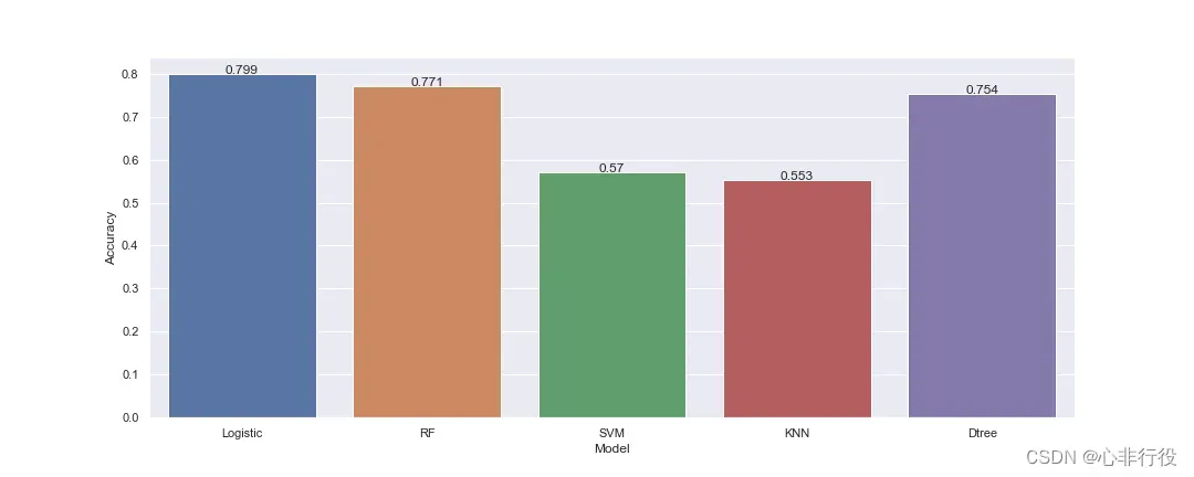
5.6 5种模型对比
>>>import seaborn as sns
>>>import matplotlib.pyplot as plt
>>>sns.set(rc={'figure.figsize':(15,6)})
>>>accuracys = [accuracy_lr, accuracy_rfc, accuracy_svm, accuracy_knn, accuracy_dtree]
>>>models = ['Logistic', 'RF', 'SVM', 'KNN', 'Dtree']
>>>bar = sns.barplot(x=models, y=accuracys)
# 显示数值标签
>>>for x, y in enumerate(accuracys):
>>>    plt.text(x, y, '%s'% round(y,3), ha='center')
>>>plt.xlabel("Model")
>>>plt.ylabel("Accuracy")
>>>plt.savefig(r"D:\data\python\exercise\test2\3.png")
>>>plt.show()
6. 预测模型
6.1 逻辑回归模型
>>>pred_lr = model_lr.predict(pred_x)
>>>pred_lr = pred_lr.astype(int)
>>>passenger_id = test_data.iloc[:, 0]
#逻辑回归的预测结果
>>>preddf1 = pd.DataFrame({'PassengerId': passenger_id,'Survived': pred_lr})
>>>preddf1.to_csv(r'D:\data\python\taitanic\titanic_pred_model_lr.csv', index=False)
6.2 随机森林
>>>pred_rfc = model_rfc.predict(pred_x)
>>>pred_rfc = pred_rfc.astype(int)
#随机森林的预测结果
>>>preddf2 = pd.DataFrame({'PassengerId': passenger_id,'Survived': pred_rfc})
>>>preddf2.to_csv(r'D:\data\python\taitanic\titanic_pred_model_rfc.csv', index=False)
6.3 支持向量机
>>>pred_svm = model_svm.predict(pred_x)
>>>pred_svm = pred_svm.astype(int)
#支持向量机的预测结果
>>>preddf3 = pd.DataFrame({'PassengerId': passenger_id,'Survived': pred_svm})
>>>preddf3.to_csv(r'D:\data\python\taitanic\titanic_pred_model_svm.csv', index=False)
6.4 K最近邻
>>>pred_knn = model_knn.predict(pred_x)
>>>pred_knn = pred_knn.astype(int)
#K最近邻分类器的预测结果
>>>preddf4 = pd.DataFrame({'PassengerId': passenger_id,'Survived': pred_knn})
>>>preddf4.to_csv(r'D:\data\python\taitanic\titanic_pred_model_knn.csv', index=False)
6.5 决策树
>>>pred_dtree= model_dtree.predict(pred_x)
>>>pred_dtree = pred_dtree.astype(int)
#决策树模型的预测结果
>>>preddf5 = pd.DataFrame({'PassengerId': passenger_id,'Survived': pred_dtree})
>>>preddf5.to_csv(r'D:\data\python\taitanic\titanic_pred_model_dtree.csv', index=False)
6.6 将上述结果交至kaggle进行评分
得到结果如下
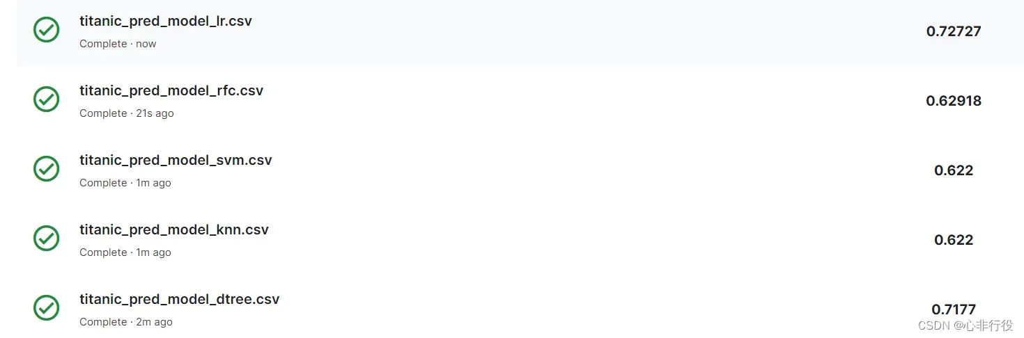
可以看到逻辑回归的分数依然是最高的
7. 完整代码
建议使用jupyter notebook完成以下内容
import numpy as np
import pandas as pd
import matplotlib.pyplot as plt
import seaborn as sns
import random

from sklearn.linear_model import LogisticRegression # 逻辑回归
from sklearn.ensemble import RandomForestClassifier # 随机森林
from sklearn.svm import SVC # 支持向量机
from sklearn.neighbors import KNeighborsClassifier # K最近邻
from sklearn.tree import DecisionTreeClassifier # 决策树

from sklearn.model_selection import train_test_split
from sklearn.linear_model import LogisticRegression
#训练数据集
train_data = pd.read_csv(r"D:\data\python\taitanic\train.csv")
#测试数据集
test_data = pd.read_csv(r"D:\data\python\taitanic\test.csv")
print('训练数据集:', train_data.shape, '测试数据集:', test_data.shape)

train_data.isnull().sum()

plt.figure(figsize=(10,5),dpi=100)
train_data['Embarked'].value_counts().plot(kind='bar')
plt.savefig(r"D:\data\python\exercise\test2\1.png")

#选取频率最高的填充到空白数据中
train_data['Embarked'] = train_data['Embarked'].fillna('S')
train_data.isnull().sum()

#处理空白年龄(Age),使用平均值填充
train_data['Age'] = train_data['Age'].fillna(int(train_data['Age'].mean()))
train_data.isnull().sum()

#至此除了Cabin(船舱号)其他缺失值已经补充完毕.Cabin这一列数据值缺失过多选择填充会导致得到的数据过于片面,因此,选择删去这一列
train_data.drop(columns = 'Cabin', axis=1,inplace=True)

train_data.head()

#处理用户阶级
pclassdf1 = pd.DataFrame()
#使用get_dummies进行one-hot编码,列名前缀是Pclass
pclassdf1 = pd.get_dummies( train_data['Pclass'] , prefix='Pclass' )
train_data = pd.concat([train_data, pclassdf1], axis=1)
train_data.drop('Pclass',axis=1, inplace=True)
train_data.head()

def gettitle(name):
    str1 = name.split(',')[1] #Mr. Owen Harris
    str2 = str1.split('.')[0]#Mr
    str3 = str2.strip()
    return str3
#存放提取后的特征
titledf1 = pd.DataFrame()
#map函数:对Series每个数据应用自定义的函数计算
titledf1['Title'] = train_data['Name'].map(gettitle)
#查看titledf的种类
titledf1['Title'].value_counts()

#姓名中头衔字符串与定义头衔类别的对应关系
title_mapdict = {
                    "Capt":       "Officer",
                    "Col":        "Officer",
                    "Major":      "Officer",
                    "Jonkheer":   "Royalty",
                    "Don":        "Royalty",
                    "Sir":        "Royalty",
                    "Dr":         "Officer",
                    "Rev":        "Officer",
                    "the Countess":"Royalty",
                    "Dona":       "Royalty",
                    "Mme":        "Mrs",
                    "Mlle":       "Miss",
                    "Ms":         "Mrs",
                    "Mr":         "Mr",
                    "Mrs":        "Mrs",
                    "Miss":       "Miss",
                    "Master":     "Master",
                    "Lady":       "Royalty"
                    }
#map函数:对Series每个数据应用自定义的函数计算
titledf1['Title'] = titledf1['Title'].map(title_mapdict)
#使用get_dummies进行one-hot编码
titledf1 = pd.get_dummies(titledf1['Title'])
train_data = pd.concat([train_data, titledf1], axis=1)
train_data.drop('Name',axis=1, inplace=True)
train_data.head()

#处理性别
sex_mapdict = {'male': 1, 'female': 0}
#map函数:对Series每个数据应用自定义的函数计算
train_data['Sex'] = train_data['Sex'].map(sex_mapdict)
sexdf1 = pd.DataFrame()
#使用get_dummies进行one-hot编码,产生虚拟变量(dummy variables),列名前缀是Sex
sexdf1 = pd.get_dummies( train_data['Sex'], prefix='Sex')
train_data = pd.concat([train_data, sexdf1], axis=1)
train_data.drop('Sex',axis=1, inplace=True)
train_data.head()

plt.figure(figsize=(18,4))
train_data['Age']=train_data['Age'].astype(np.int)
average_age=train_data[['Age','Survived']].groupby('Age',as_index=False).mean()
sns.barplot(x='Age',y='Survived',data=average_age,palette='BuPu')
plt.savefig(r"D:\data\python\exercise\test2\2.png")

agedf1 = pd.DataFrame(train_data['Age'])
agedf1['Age_baby'] = agedf1['Age'].map(lambda s: 1 if 0 <= s < 15 else 0)
agedf1['Age_youth'] = agedf1['Age'].map(lambda s: 1 if 15 <= s < 35 else 0)
agedf1['Age_middle'] = agedf1['Age'].map(lambda s: 1 if 35 <= s <=60 else 0)
agedf1['Age_old'] = agedf1['Age'].map(lambda s: 1 if 60 <= s else 0)
train_data = pd.concat([train_data,agedf1], axis=1)
train_data.drop('Age',axis=1, inplace=True)
train_data.head()

#存放家庭信息
familydf1 = pd.DataFrame()

#家庭人数
familydf1['FamilySize'] = train_data['Parch'] + train_data['SibSp'] + 1

#家庭类别
#if 条件为真的时候返回if前面内容,否则返回0
familydf1['Family_Single'] = familydf1['FamilySize'].map(lambda s: 1 if s == 1 else 0)

familydf1['Family_Small'] = familydf1['FamilySize'].map(lambda s: 1 if 2 <= s <= 4 else 0)

familydf1['Family_Large'] = familydf1['FamilySize'].map(lambda s: 1 if 5 <= s else 0)
familydf1.drop('FamilySize',axis=1, inplace=True)
train_data = pd.concat([train_data, familydf1], axis=1)
train_data.drop('Parch',axis=1, inplace=True)
train_data.drop('SibSp',axis=1, inplace=True)
train_data.head()

#船票在这里没什么用处,选择删除
train_data.drop('Ticket',axis=1, inplace=True)

faredf1=pd.DataFrame(train_data['Fare'])
faredf1['Fare_First']=faredf1['Fare'].map(lambda f: 1 if f >= 30 and f <= 870 else 0)
faredf1['Fare_Second']=faredf1['Fare'].map(lambda f: 1 if f >= 12 and f < 30 else 0)
faredf1['Fare_Third']=faredf1['Fare'].map(lambda f: 1 if f >= 3 and f < 12 else 0)
train_data = pd.concat([train_data,faredf1], axis=1)
train_data.drop('Fare',axis=1, inplace=True)
train_data.head()

#处理上船港口
embarkeddf1 = pd.DataFrame()
#使用get_dummies进行one-hot编码,产生虚拟变量(dummy variables),列名前缀是Embarked
embarkeddf1 = pd.get_dummies(train_data['Embarked'], prefix='Embarked')
train_data = pd.concat([train_data, embarkeddf1], axis=1)
train_data.drop('Embarked',axis=1, inplace=True)
train_data.head()

test_data.isnull().sum()

#处理测试集数据
test_data['Age'] = test_data['Age'].fillna(int(test_data['Age'].mean()))
test_data['Fare'] = test_data['Fare'].fillna(test_data['Fare'].mean())
test_data.drop(columns = 'Cabin', axis=1,inplace=True)
test_data.isnull().sum()

agedf2 = pd.DataFrame(test_data['Age'])
agedf2['Age_baby'] = agedf2['Age'].map(lambda s: 1 if 0 <= s < 15 else 0)
agedf2['Age_youth'] = agedf2['Age'].map(lambda s: 1 if 15 <= s < 35 else 0)
agedf2['Age_middle'] = agedf2['Age'].map(lambda s: 1 if 35 <= s <=60 else 0)
agedf2['Age_old'] = agedf2['Age'].map(lambda s: 1 if 60 <= s else 0)
test_data = pd.concat([test_data, agedf2], axis=1)
test_data.drop('Age',axis=1, inplace=True)
#处理性别
test_data['Sex'] = test_data['Sex'].map(sex_mapdict)
sexdf2 = pd.DataFrame()
sexdf2 = pd.get_dummies( test_data['Sex'], prefix='Sex')
test_data = pd.concat([test_data, sexdf2], axis=1)
test_data.drop('Sex',axis=1, inplace=True)
#处理上船港口
embarkeddf2 = pd.DataFrame()
embarkeddf2 = pd.get_dummies(test_data['Embarked'], prefix='Embarked')
test_data = pd.concat([test_data, embarkeddf2], axis=1)
test_data.drop('Embarked',axis=1, inplace=True)
#处理用户阶级
pclassdf2 = pd.DataFrame()
pclassdf2 = pd.get_dummies( test_data['Pclass'] , prefix='Pclass' )
test_data = pd.concat([test_data, pclassdf2], axis=1)
test_data.drop('Pclass',axis=1, inplace=True)
#存放提取后的特征
titledf2 = pd.DataFrame()
titledf2['Title'] = test_data['Name'].map(gettitle)
titledf2['Title'] = titledf2['Title'].map(title_mapdict)
titledf2 = pd.get_dummies(titledf2['Title'])
test_data = pd.concat([test_data, titledf2], axis=1)
test_data.drop('Name',axis=1, inplace=True)
#存放家庭信息
familydf2 = pd.DataFrame()
familydf2['FamilySize'] = test_data['Parch'] + test_data['SibSp'] + 1
familydf2['Family_Single'] = familydf2['FamilySize'].map(lambda s: 1 if s == 1 else 0)
familydf2['Family_Small'] = familydf2['FamilySize'].map(lambda s: 1 if 2 <= s <= 4 else 0)
familydf2['Family_Large'] = familydf2['FamilySize'].map(lambda s: 1 if 5 <= s else 0)
familydf2.drop('FamilySize',axis=1, inplace=True)
test_data = pd.concat([test_data, familydf2], axis=1)
test_data.drop('Parch',axis=1, inplace=True)
test_data.drop('SibSp',axis=1, inplace=True)
#处理船票
faredf2=pd.DataFrame(test_data['Fare'])
faredf2['Fare_First']=faredf2['Fare'].map(lambda f: 1 if f >= 30 and f <= 870 else 0)
faredf2['Fare_Second']=faredf2['Fare'].map(lambda f: 1 if f >= 12 and f < 30 else 0)
faredf2['Fare_Third']=faredf2['Fare'].map(lambda f: 1 if f >= 3 and f < 12 else 0)
test_data = pd.concat([test_data, faredf2], axis=1)
test_data.drop('Fare',axis=1, inplace=True)
test_data.drop('Ticket',axis=1, inplace=True)
test_data.head()

corrdf = train_data.corr()
corrdf

corrdf['Survived'].round(4).abs().sort_values(ascending=False)

source_y = train_data.Survived
source_x = train_data.drop(['Survived'],axis=1)
train_x, test_x, train_y, test_y = train_test_split(source_x,
           source_y , train_size=0.8,test_size=0.2)

pred_x=test_data

model_lr = LogisticRegression()
model_lr.fit(train_x, train_y)
pred_lr = model_lr.predict(pred_x)
pred_lr = pred_lr.astype(int)
accuracy_lr = model_lr.score(test_x,test_y)
print("逻辑回归的测试结果:", accuracy_lr)

model_rfc = RandomForestClassifier()
model_rfc.fit(train_x, train_y)
pred_rfc = model_rfc.predict(pred_x)
pred_rfc = pred_rfc.astype(int)
accuracy_rfc = model_rfc.score(test_x,test_y)
print("随机森林的预试结果:", accuracy_rfc)

model_svm = SVC()
model_svm.fit(train_x, train_y)
pred_svm = model_svm.predict(pred_x)
pred_svm = pred_svm.astype(int)
accuracy_svm = model_svm.score(test_x,test_y)
print("支持向量机的测试结果:", accuracy_svm)

model_knn = KNeighborsClassifier()
model_knn.fit(train_x, train_y)
pred_knn = model_knn.predict(pred_x)
pred_knn = pred_knn.astype(int)
accuracy_knn = model_knn.score(test_x,test_y)
print("K最近邻分类器的测试结果:", accuracy_knn)

model_dtree = DecisionTreeClassifier()
model_dtree.fit(train_x, train_y)
pred_dtree= model_dtree.predict(pred_x)
pred_dtree = pred_dtree.astype(int)
accuracy_dtree= model_dtree.score(test_x,test_y)
print("决策树模型的测试结果:", accuracy_dtree)

import seaborn as sns
import matplotlib.pyplot as plt

sns.set(rc={'figure.figsize':(15,6)}) # 设置画布大小
accuracys = [accuracy_lr, accuracy_rfc, accuracy_svm, accuracy_knn, accuracy_dtree]
models = ['Logistic', 'RF', 'SVM', 'KNN', 'Dtree']
bar = sns.barplot(x=models, y=accuracys)

# 显示数值标签
for x, y in enumerate(accuracys):
    plt.text(x, y, '%s'% round(y,3), ha='center')

plt.xlabel("Model")
plt.ylabel("Accuracy")
plt.savefig(r"D:\data\python\exercise\test2\3.png")
plt.show()

#数据框:乘客id,预测生存情况的值
passenger_id = test_data.iloc[:, 0]
#逻辑回归的预测结果
preddf1 = pd.DataFrame({'PassengerId': passenger_id,'Survived': pred_lr})
preddf1.to_csv(r'D:\data\python\taitanic\titanic_pred_model_lr.csv', index=False)
#随机森林的预测结果
preddf2 = pd.DataFrame({'PassengerId': passenger_id,'Survived': pred_rfc})
preddf2.to_csv(r'D:\data\python\taitanic\titanic_pred_model_rfc.csv', index=False)
#支持向量机的预测结果
preddf3 = pd.DataFrame({'PassengerId': passenger_id,'Survived': pred_svm})
preddf3.to_csv(r'D:\data\python\taitanic\titanic_pred_model_svm.csv', index=False)
#K最近邻分类器的预测结果
preddf4 = pd.DataFrame({'PassengerId': passenger_id,'Survived': pred_knn})
preddf4.to_csv(r'D:\data\python\taitanic\titanic_pred_model_knn.csv', index=False)
#决策树模型的预测结果
preddf5 = pd.DataFrame({'PassengerId': passenger_id,'Survived': pred_dtree})
preddf5.to_csv(r'D:\data\python\taitanic\titanic_pred_model_dtree.csv', index=False)
8. 总结
以上就是泰坦尼克号的生存预测分析。
如果你觉得这篇文章对你有用,建议点赞收藏。
欢迎各位读者指正错误,请在评论区留言。或者发表自己的看法,小编不胜感激。
文章出处登录后可见!
已经登录?立即刷新